Algorithms

The algorithms module is split into two main submodules. On the one hand, PrimitiveAlgorithms handle fundamental quantum operations such as expectation values, overlaps, transition amplitudes, and sampling. On the other hand, CompositeAlgorithms provide black-box implementations of complete quantum algorithms that orchestrate multiple primitives. This section covers both types of algorithms.

Primitive Algorithms

Primitive Algorithms are the building blocks for quantum computation in OpenQARP. They encapsulate single quantum measurement operations and automatically detect the appropriate computation target based on the input arguments (bra, ket, and operator). The .target attribute indicates which type of computation is being performed.

The following table describes the available targets and their corresponding PrimitiveAlgorithms:

Target	Formula	Available PrimitiveAlgorithm
Sampling	Raw measurement distribution \(P(\mathbf{x}) = |\langle \mathbf{x} | \psi \rangle|^2\)	Sampler
Expectation value	\(\langle \psi | O | \psi \rangle\) or \(|\langle \psi | O | \psi \rangle|^2\)	StateVector, HadamardTest, TermwiseHadamardTest, MirrorTest (squared), SWAPTest (squared), InterferometricTest, CuttingPrimitive, PauliAveraging
Overlap	\(\langle \phi | \psi \rangle\) or \(|\langle \phi | \psi \rangle|^2\)	StateVector, HadamardTest, MirrorTest (squared), SWAPTest (squared), TermwiseSWAPTest (squared)
Transition amplitude	\(\langle \phi | O | \psi \rangle\) or \(|\langle \phi | O | \psi \rangle|^2\)	StateVector, HadamardTest, MirrorTest (squared), SWAPTest (squared)

Target Detection

The PrimitiveAlgorithm automatically determines the target based on the provided arguments:

• Sampling: Only ket is provided (no bra or operator)

• Expectation value: ket and operator provided, bra equals ket or is omitted

• Overlap: bra and ket provided, no operator

• Transition amplitude: All three (bra, operator, ket) are provided

Now, we list one by one, each of the approaches available in OpenQARP:

Sampler

The Sampler primitive is used to execute a quantum circuit and collect raw measurement statistics. Unlike other primitives that compute specific targets (expectation values, overlaps, etc.), the Sampler simply runs the circuit and returns the measurement outcome distribution. This is particularly useful for algorithms that require raw measurement data, such as Quantum Phase Estimation (QPE), where the phase information is encoded in the measurement frequencies.

\[P(\mathbf{x}) = |\langle \mathbf{x} | \psi \rangle|^2\]

The Sampler automatically sets the target to Target.SAMPLING since only a ket block is provided (no bra or operator).

The following code demonstrates how to use the Sampler to collect measurement statistics from a quantum circuit:

from qarp.algorithms import Sampler
from qarp.blocks import SimpleBlock
from qarp.engines import QarpEngine

# Create a simple circuit that prepares a Bell state
block = SimpleBlock(2, name="bell")
block.h(0)
block.cx(0, 1)

# Create and build the Sampler
sampler = Sampler(ket=block, n_shots=1000).build()

# Run the Sampler to collect measurement statistics
my_engine = QarpEngine()
my_engine.build([sampler])

result = my_engine.run()
print("Measurement distribution:", result[0])
# Expected output: approximately {(0, 0): 0.5, (1, 1): 0.5}

The Sampler returns a dictionary mapping measurement outcomes (as tuples) to their observed probabilities, normalised by the number of shots.

StateVector

While statevector simulation is not exactly an algorithm, it does fit the concept of PrimitiveAlgorithm described before, and is a useful tool for proof of concept calculations and for checking results you obtain from devices or other measurement approaches. The API for the StateVector object is very simple:

The reason that the StateVector object does not take a shots argument in the constructor is that the number of shots is ill-defined as no practical measurement circuits are generated, and for the same reason a device argument is equally redundant.

Reusing the block prepared above, and given a qubit operator, we can instantiate the StateVector algorithm object.

from qarp.algorithms import StateVector
from qarp.operators import QubitOperator

ham = QubitOperator("Z0 Z1")
sv = StateVector(bra=block, operator=ham, ket=block)

In the previous example, the same block was provided for both bra and ket attributes. Thus, an expectation value will be computed using StateVector approach. To carry on the computation, an engine is needed. Please, check qarp.engines doc pages to see a more detailed example.

The observable is never materialised as a matrix. On QarpEngine the contraction ⟨bra|H|ket⟩ runs in C++ (QarpSimulator.transition): the Pauli terms are grouped by their X/Y flip pattern and the whole sum is evaluated in one pass over the two statevectors, so a 2000-term molecular Hamiltonian at 20 qubits costs about 0.1 s on a laptop. Z-only observables (Ising / MaxCut costs) use a cached diagonal instead. A simulator that only provides statevector (the GPU engine’s host path, third-party backends) falls back to the numpy sweep qarp.algorithms._primitives.state_vector.pauli_expectation with the same result.

(Termwise) HadamardTest

The Hadamard test is a well known approach for evaluating various terms of interest, and the first of the algorithms that accepts a shot-based simulation as part of the approach. Here we can find HadamardTest and its termwise approach TermwiseHadamardTest which can handle a Hamiltonian with more than one term.

This approach is able to estimate the real or imaginary part of the expectation value of a unitary operator with respect to a quantum state. It is particularly useful for computing overlaps and transition amplitudes between quantum states. The method involves preparing an ancillary qubit in a superposition state using a Hadamard gate, entangling it with the target quantum system via controlled operations, and then measuring the ancilla to extract the desired information.

\[\text{Re}(\langle \psi | U | \psi \rangle), \quad \text{Im}(\langle \psi | U | \psi \rangle)\]

Since OpenQARP is built in a blockwise structure, the inputs of this PrimitiveAlgorithm requires Block objects. OpenQARP provides functionalities for transforming a QubitOperator into a Block structure. They are called Factories. The following code uses HadamardTest to compute the expectation value of a system, where the original Hamiltonian is encoded as a QubitOperator.

from qarp.factories import PauliBlockFactory
from qarp.algorithms import HadamardTest
from qarp.blocks import SimpleBlock
from qarp.operators import QubitOperator
from qarp.engines import QarpEngine

ham = QubitOperator("Z0 Z1 Z2")
ham_block = PauliBlockFactory.from_qubit_operator(ham, n_qubits=4)
block = SimpleBlock(4, name="ghz")
block.h(0)
block.cx(0, 1)
block.cx(1, 2)
block.cx(2, 3)

meas = HadamardTest(bra=block, operator=ham_block[0], ket=block).build()

# Run the HadamardTest to compute the expectation value of the above operator on the GHZ state.
my_engine = QarpEngine()
my_engine.build([meas])

result = my_engine.run()
print("Result:", result[0])

However, in some cases a Hamiltonian is composed of more than one term with different coefficients. The following code showcases such a case, in which a TermwiseHadamardTest is more convenient.

from qarp.algorithms import TermwiseHadamardTest
from qarp.blocks import SimpleBlock
from qarp.operators import QubitOperator
from qarp.engines import QarpEngine

ham = QubitOperator("Z0 Z1 Z2") + .5 * QubitOperator("X2 X3")
block = SimpleBlock(4, name="ghz")
block.h(0)
block.cx(0, 1)
block.cx(1, 2)
block.cx(2, 3)

# Pass the QubitOperator straight to TermwiseHadamardTest: it expands the
# terms into per-term blocks and weights each by its coefficient magnitude
# (here 1.0 and 0.5).  Building the blocks yourself and passing them as a
# list instead would require handing over the magnitudes via ``coefficients=``.
meas = TermwiseHadamardTest(bra=block, operator=ham, ket=block).build()

# Run the TermwiseHadamardTest to compute the expectation value
# of the above combination of operators on the GHZ state.
my_engine = QarpEngine()
my_engine.build([meas])

result = my_engine.run()
print("Result:", result[0])

Note that both HadamardTest and TermwiseHadamardTest allow you to set a custom Device and a given number of shots for the shot simulation. It is also worth noting that the default behavior if a QubitOperator object is passed as the operator argument to the TermwiseHadamardTest then the PauliBlockFactory is called under the hood.

(Termwise) SWAPTest

The SWAP Test is a quantum algorithm used to estimate the squared overlap between two quantum states, which is particularly useful for determining their similarity. It operates by preparing a controlled SWAP operation between two quantum registers and an ancillary qubit, followed by a Hadamard transformation and measurement of the ancilla. The probability of measuring the ancilla in the zero state is directly related to the squared overlap of the input states. Here we can find SWAPTest and its termwise approach TermwiseSWAPTest which can handle multiple bra states simultaneously.

\[|\langle \phi | \psi \rangle|^2, \quad |\langle \phi | U | \psi \rangle|^2\]

Key Features:

• Overlap estimation: Compute \(|\langle \phi | \psi \rangle|^2\) between two quantum states

• Transition amplitude: When an operator is provided, computes \(|\langle \phi | U | \psi \rangle|^2\)

• Hardware friendly: Only requires controlled-SWAP operations and single-qubit measurements

• Shot-based: Supports execution on real quantum devices with configurable shots

In OpenQARP, the SWAP Test is implemented as a PrimitiveAlgorithm that can be applied to expressions such as Overlap and TransitionAmplitude. This method is especially valuable in scenarios where direct access to the full state vector is limited, and it enables efficient evaluation of quantum state fidelity on both simulators and real quantum devices.

The following code shows an example of computing the overlap between two quantum states using SWAPTest:

from qarp.algorithms import SWAPTest
from qarp.blocks import SimpleBlock
from qarp.engines import QarpEngine

block1 = SimpleBlock(4, name="block1")
block1.h(0)
block1.cx(0, 1)
block1.cx(1, 2)
block1.cx(2, 3)

block2 = SimpleBlock(4, name="block2")
block2.h(0)
block2.h(1)
block2.cx(0, 1)
block2.cx(1, 2)
block2.cx(2, 3)

meas = SWAPTest(bra=block1, ket=block2, n_shots=10000).build()

# Run the SWAPTest between block1 and block2.
my_engine = QarpEngine()
my_engine.build([meas])

result = my_engine.run()
print("Squared overlap:", result[0])

To compute a transition amplitude squared \(|\langle \phi | U | \psi \rangle|^2\), provide an operator:

from qarp.algorithms import SWAPTest
from qarp.blocks import SimpleBlock
from qarp.factories import PauliBlockFactory
from qarp.operators import QubitOperator

bra = SimpleBlock(4, name="bra")
bra.h(0)
bra.cx(0, 1)
bra.cx(1, 2)
bra.cx(2, 3)

ket = SimpleBlock(4, name="ket")
ket.x(0)
ket.x(1)

# Define a unitary operator
op = QubitOperator("X0 X1")
op_block = PauliBlockFactory.from_qubit_operator(op, n_qubits=4)[0]

meas = SWAPTest(bra=bra, operator=op_block, ket=ket).build()

TermwiseSWAPTest extends this functionality to handle multiple bra states at once, computing the sum of squared overlaps:

from qarp.algorithms import TermwiseSWAPTest
from qarp.blocks import SimpleBlock
from qarp.engines import QarpEngine

block1 = SimpleBlock(4, name="block1")
block1.h(0)
block1.cx(0, 1)
block1.cx(1, 2)
block1.cx(2, 3)

block2 = SimpleBlock(4, name="block2")
block2.h(0)
block2.h(1)
block2.cx(0, 1)
block2.cx(1, 2)
block2.cx(2, 3)

block3 = SimpleBlock(4, name="block3")
block3.h(0)
block3.h(1)
block3.cx(0, 1)
block3.cx(1, 2)
block3.cx(2, 3)

meas = TermwiseSWAPTest(bra=[block1, block2], ket=block3).build()

# Run the TermwiseSWAPTest to compute the sum of the overlaps
# between block1 with block3 and block2 with block3.
my_engine = QarpEngine()
my_engine.build([meas])

result = my_engine.run()
print("Result:", result[0])

Note that both SWAPTest and TermwiseSWAPTest allow you to set a custom Device and a given number of shots for the shot simulation.

Also, TermwiseSWAPTest allows a set of coefficients to be passed as weights for each term.

coeffs = [0.3, 0.8]
meas = TermwiseSWAPTest(bra=[block1, block2], ket=block3, coefficients=coeffs).build()

# Run the TermwiseSWAPTest to compute the weighted overlaps.
my_engine = QarpEngine()
my_engine.build([meas])

result = my_engine.run()
print("Result:", result[0])

MirrorTest

The Mirror Test is a quantum measurement technique used to estimate the squared magnitude of overlaps or expectation values, such as │⟨ψ|O|ψ⟩│² or │⟨ϕ|ψ⟩│². Unlike the Hadamard or SWAP Tests, which provide direct access to real or imaginary components, the Mirror Test focuses on computing the absolute square of complex amplitudes. This is achieved by constructing a mirrored quantum circuit that duplicates the original computation and interferes the two paths to extract the desired quantity.

\[|\langle \psi | O | \psi \rangle|^2, \quad |\langle \phi | \psi \rangle|^2, \quad |\langle \phi | O | \psi \rangle|^2\]

In OpenQARP, the Mirror Test is implemented as a PrimitiveAlgorithm and is particularly useful in scenarios where the squared value of a quantum observable is of interest, such as fidelity estimation or transition probability analysis.

The following code showcases an example in which we compute the square of the expectation value of a quantum system.

from qarp.factories import PauliBlockFactory
from qarp.algorithms import MirrorTest
from qarp.blocks import SimpleBlock
from qarp.operators import QubitOperator
from qarp.engines import QarpEngine

ham = QubitOperator("Z0 Z1 Z2")
ham_block = PauliBlockFactory.from_qubit_operator(ham, n_qubits=4)
block = SimpleBlock(4, name="ghz")
block.h(0)
block.cx(0, 1)
block.cx(1, 2)
block.cx(2, 3)

meas = MirrorTest(bra=block, operator=ham_block[0], ket=block).build()

# Run the MirrorTest to compute the squared expectation value of the above operator on the GHZ state.
my_engine = QarpEngine()
my_engine.build([meas])

result = my_engine.run()
print("Result:", result[0])

Note that when running meas in an Engine, the returned result will be the square of the expectation value.

InterferometricTest

The Interferometric Test is a quantum measurement technique that leverages interference patterns to extract information about quantum states and operators. It is particularly suited for evaluating expectation values and transition amplitudes by encoding the computation into an interferometric setup, where the phase differences between quantum paths reveal the desired quantities. This method is advantageous in scenarios requiring high precision or when working with hardware that supports interferometric operations.

Unlike the SWAP Test or Mirror Test which compute squared quantities, the Interferometric Test can estimate the complex expectation value directly, providing both real and imaginary parts:

\[\text{Re}(\langle \psi | O | \psi \rangle), \quad \text{Im}(\langle \psi | O | \psi \rangle)\]

Key Features:

• Complex value estimation: Can compute both real and imaginary parts of expectation values

• Configurable components: Choose which parts to estimate via real=True/False and imaginary=True/False

• Flexible sampling backend: Uses either MirrorTest or SWAPTest as the underlying sampling algorithm

• Reference state: Currently uses the all-zero state as reference (requires ket to be orthogonal to it)

The following code shows the expectation value computation using the Interferometric Test:

from qarp.factories import PauliBlockFactory
from qarp.algorithms import InterferometricTest, MirrorTest
from qarp.blocks import ComputationalBasisStateBlock
from qarp.operators import QubitOperator
from qarp.engines import QarpEngine

# Define a Hamiltonian and convert to block
ham = QubitOperator("Z0 Z1 Z2")
ham_block = PauliBlockFactory.from_qubit_operator(ham, n_qubits=4)

# Prepare a computational basis state (must not be all-zeros)
block = ComputationalBasisStateBlock([0, 1, 1, 1])

# Build the InterferometricTest
meas = InterferometricTest(
    bra=block,
    operator=ham_block[0],
    ket=block,
    real=True,
    imaginary=True,
    sampling_algorithm=MirrorTest()
).build()

# Run the InterferometricTest
my_engine = QarpEngine()
my_engine.build([meas])

result = my_engine.run()
print("Result:", result[0])  # Returns complex value

You can also use the SWAPTest as the underlying sampling algorithm:

from qarp.algorithms import InterferometricTest, SWAPTest

meas = InterferometricTest(
    bra=block,
    operator=ham_block[0],
    ket=block,
    sampling_algorithm=SWAPTest()
).build()

Note

The InterferometricTest requires the ket state to be a ComputationalBasisStateBlock and must not be the all-zero state, as this serves as the reference state for the interferometric measurement.

CuttingPrimitive

The CuttingPrimitive implements gate-cutting techniques. It is engine-agnostic. See the qarp.cutting documentation for the full pipeline and the standalone QPDDecomposition path.

Pauli Averaging

PauliAveraging allows you to compute expectation values \(\langle \psi | O | \psi \rangle\) while taking advantage of a qarpx-native commuting-Pauli grouping to reduce the total number of measurement circuits and shots required. The default strategy, FullyCommuting, groups by general commutation; QubitWiseCommuting is available through the grouping argument.

from qarp.algorithms import PauliAveraging
from qarp.operators import QubitOperator
from qarp.engines import QarpEngine
from qarp.blocks import ComputationalBasisStateBlock

state_block = ComputationalBasisStateBlock([1, 1, 0, 1])
op = QubitOperator("Z0 Z1")  - QubitOperator("Z2 Z3") + QubitOperator("Z0 Y1 X3")
m = PauliAveraging(bra=state_block, operator=op, ket=state_block)
engine = QarpEngine()
engine.build([m])
engine.run()

Classical Shadows

PauliShadow runs one state-agnostic randomized-measurement campaign and lets you estimate many observables from that single dataset, at a cost set by each observable’s shadow norm rather than by the number of observables or qubits (Huang–Kueng–Preskill, 2020). It is an ordinary primitive — engine.run returns the bound operator’s expectation — and it also exposes the raw snapshots as a reusable shadow.dataset for estimating further observables without re-collecting.

For a single, fixed Hamiltonian, PauliAveraging is more shot-efficient; reach for shadows when you want many/unknown local observables from one campaign.

from qarp.algorithms import PauliShadow
from qarp.blocks import SimpleBlock
from qarp.engines import QarpEngine
from qarp.operators import QubitOperator

ket = SimpleBlock(2)
ket.h(0)
ket.cx(0, 1)

shadow = PauliShadow(QubitOperator("Z0 Z1"), ket, n_settings=2000, seed=0)
engine = QarpEngine(seed=1)
engine.build([shadow])
zz = engine.run()[0]                       # <Z0 Z1>

est = shadow.dataset.estimator()           # reuse the same campaign ...
xx = est.expval("X0 X1").value             # ... for another observable, no re-run

The estimator uses median-of-means; each expval returns a ShadowEstimate carrying the value and error, the accuracy half-width \(\varepsilon = \sqrt{34\,\hat{V}/N}\) of Huang–Kueng–Preskill Theorem 1 — the \(\varepsilon\) for which \(\Pr[\,|\text{value} - \text{true}| \ge \varepsilon\,] \le \delta\) at the delta that fixed the batch count, with \(\hat{V}\) the empirical single-setting variance and \(N\) the per-batch size. It is a worst-case bound carrying the paper’s own deliberately loose constant 34, so it typically sits several times above the scatter you observe between repeats: read it as a guarantee, not as a standard error. Only the random-Pauli ensemble ships today; matchgate and global-Clifford ensembles are planned as additional kernels.

Composite Algorithms

Composite algorithms are higher-level workflows that combine quantum circuits, primitive measurements, and classical post-processing. Depending on the method, a workflow may include an optimization loop, iterative refinement, repeated sampling, or several stages of circuit construction and execution.

Concrete composite algorithms inherit from CompositeAlgorithm and provide two main operations:

• build() constructs and configures the circuits, primitives, and other resources required by the algorithm.

• run() executes the workflow and returns or stores its algorithm-specific result.

Constructor options and return values are specific to each algorithm. Many algorithms accept an execution engine or a measurement primitive, while variational methods may additionally accept an optimizer, a gradient option, or verbosity controls. Their defaults and compatibility requirements are not uniform, so consult the relevant algorithm section or API reference rather than assuming that an option is shared by every composite algorithm.

Amplitude Amplification

Amplitude amplification increases the probability of measuring a designated good subspace. Given a preparation \(A\) with initial good-state probability \(\sin^2(\theta)\), one amplification iterate changes that probability according to

\[P_k(\mathrm{good}) = \sin^2((2k + 1)\theta),\]

after \(k\) iterations. OpenQARP implements the phase-exact iterate

\[Q = A R_0 A^\dagger O_\mathrm{good},\]

where \(R_0 = 2|0\ldots0\rangle\langle0\ldots0| - I\) and the caller’s oracle must implement exactly \(O_\mathrm{good} = I - 2\Pi_\mathrm{good}\). The algorithm requires an explicit non-negative iteration count; it does not infer one from an opaque oracle.

This convention follows Brassard, Hoyer, Mosca, and Tapp, Quantum Amplitude Amplification and Estimation, Eq. (1). Their operator is \(Q=-A S_0 A^{-1}S_\chi\), with \(S_0=I-2|0\rangle\langle0|\). Since OpenQARP’s ReflectionBlock is \(R_0=-S_0\), this becomes exactly \(Q=A R_0 A^\dagger O_\mathrm{good}\). The success-probability expression above follows their Eqs. (5) and (8).

The following one-qubit example starts with good-state probability \(1/4\) and reaches probability one after a single iterate:

import numpy as np
import qarp

from qarp.algorithms import AmplitudeAmplification, Sampler
from qarp.blocks import PhaseShiftBlock, SimpleBlock

theta = np.pi / 6
state_preparation = SimpleBlock(1, name="A")
state_preparation.ry(0, 2 * theta)

# diag(1, -1): mark |1> as good.
oracle = PhaseShiftBlock(np.pi, name="O_good")

amplification = AmplitudeAmplification(
    state_preparation,
    oracle,
    n_iterations=1,
    good_states=[1],
    primitive=Sampler(n_shots=qarp.EXACT),
).build()

distribution = amplification.run()
print(distribution)
print(amplification.success_probability)
# {(1,): approximately 1.0}
# 1.0

Sampler bit tuples are LSB-first. good_states instead uses ordinary full-register integer labels; it is optional reporting metadata and does not construct or alter the oracle. If it is omitted, success_probability remains None.

Existing blocks are sufficient for common phase oracles: PhaseShiftBlock(pi) marks a one-qubit \(|1\rangle\), while X-conjugated MCZ gates can mark chosen computational-basis labels on wider registers.

The oracle contract is a promise, not a validated property: OpenQARP checks the oracle’s type and register width, but proving that an arbitrary unitary equals \(I - 2\Pi_\mathrm{good}\) would require building its dense matrix, which is exponential in the register width. The phase convention is therefore the caller’s responsibility. The one pitfall worth memorising is that a raw ReflectionBlock about the good subspace has the opposite sign, \(2\Pi-I=-(I-2\Pi)\), and must be composed with a gphase(pi) block before it can serve as a good-state oracle:

import numpy as np

from qarp.blocks import CompositeBlock, ReflectionBlock, SimpleBlock

n_qubits = 2
sign_flip = SimpleBlock(n_qubits, name="MinusIdentity")
sign_flip.gphase(np.pi)
# I - 2|0..0><0..0| : marks the all-zeros state as good.  Conjugate the
# reflection to relocate the mark.
oracle = CompositeBlock([sign_flip, ReflectionBlock(n_qubits)], n_qubits)

Omitting the sign adjustment does not change standalone measurement probabilities — sampling is blind to a global phase — but the iterate then equals \(-Q\), and the minus becomes a relative phase once a later algorithm controls the iterate: every eigenphase read by quantum amplitude estimation is silently shifted by one half.

Quantum Amplitude Estimation

Canonical quantum amplitude estimation (QAE) estimates the initial good-state probability without measuring the state register. For

\[A|0\rangle = \sqrt{1-a}|\psi_\mathrm{bad}\rangle + \sqrt{a}|\psi_\mathrm{good}\rangle,\]

write \(a=\sin^2(\theta)\). The phase-exact amplification iterate has relevant eigenphases \(\pm 2\theta\). QAE applies phase estimation to that iterate, and an estimation-register label \(y\) gives

\[\widetilde a(y) = \sin^2\left(\frac{\pi y}{2^m}\right),\]

where \(m\) is the number of estimation qubits. The two conjugate QPE peaks describe the same amplitude, so OpenQARP folds \(y\) and \(2^m-y\) together before choosing the most probable result.

The following exactly representable example estimates \(a=\sin^2(\pi/8)\):

import numpy as np
import qarp

from qarp.algorithms import AmplitudeEstimation
from qarp.algorithms import Sampler
from qarp.blocks import PhaseShiftBlock, SimpleBlock

theta = np.pi / 8
state_preparation = SimpleBlock(1, name="A")
state_preparation.ry(0, 2 * theta)
oracle = PhaseShiftBlock(np.pi, name="O_good")

estimation = AmplitudeEstimation(
    state_preparation,
    oracle,
    n_ancilla=3,
    primitive=Sampler(n_shots=qarp.EXACT),
).build()

estimate = estimation.run()
print(estimate)
print(estimation.folded_distribution)

The block layout is estimation register first, state register second. Sampler keys are LSB-first, while phase_bin is the corresponding ordinary integer label. distribution retains the raw QPE probabilities; folded_distribution combines conjugate bins, and result_probability is the selected folded bin’s complete probability mass.

The oracle must implement exactly \(O_\mathrm{good}=I-2\Pi_\mathrm{good}\). Supplying its negative shifts all controlled eigenphases by one half and makes QAE estimate the complement \(1-a\). AmplitudeEstimationBlock is measurement-free and can be embedded in larger circuits; AmplitudeEstimation samples only its estimation register. This implementation is canonical QAE, not iterative, maximum-likelihood, Bayesian, or noise-aware amplitude estimation.

Grover Search

Grover specializes amplitude amplification to uniform preparation over \(N=2^n\) basis states. Given a caller-declared number \(t\) of marked states, it sets

\[\theta=\arcsin\sqrt{t/N}, \qquad P_k(\mathrm{good})=\sin^2((2k+1)\theta),\]

and selects the better of the two non-negative integers surrounding the first continuous optimum \(\pi/(4\theta)-1/2\). The smaller count wins a numerical tie, so dense marked sets can correctly require zero oracle calls.

This four-item example marks integer label 2. OpenQARP bit tuples are LSB-first, so that label appears as (0, 1):

import qarp

from qarp.algorithms import Grover
from qarp.algorithms import Sampler
from qarp.blocks import SimpleBlock

oracle = SimpleBlock(2, name="O_good")
oracle.x(0)
oracle.mcz([0, 1])
oracle.x(0)

search = Grover(
    oracle,
    n_marked=1,
    good_states=[2],
    primitive=Sampler(n_shots=qarp.EXACT),
).build()

distribution = search.run()
print(distribution)
print(search.most_likely_states)
print(search.success_probability)

n_marked selects the iteration count but does not define or inspect the oracle. Optional good_states contains exactly n_marked unique integer labels and is reporting metadata only. When it is omitted, success_probability remains None. predicted_success_probability is the analytic probability, whereas success_probability is the measured mass on the explicitly supplied labels.

Unknown-count search, including the Boyer–Brassard–Høyer–Tapp retry schedule, is outside this implementation. The oracle sign convention is the same phase-exact \(I-2\Pi_\mathrm{good}\) contract used by amplitude amplification and QAE.

Quantum Phase Estimation (QPE)

Quantum Phase Estimation estimates the eigenphase \(\phi \in [0, 1)\) of a unitary operator. If

\[U |\psi\rangle = e^{2\pi i\phi} |\psi\rangle,\]

then QPE takes a circuit that prepares \(|\psi\rangle\) and returns a binary approximation to \(\phi\) with high probability. QPE therefore measures an eigenphase, not a Hamiltonian energy directly. For the common choice \(U=e^{-iHt}\), an energy \(E\) maps to \(\phi=(-Et/2\pi)\bmod 1\); the sign, evolution time, and phase wrapping must be accounted for when converting the measured phase back to an energy.

The QPE circuit prepares an ancilla register in superposition, applies controlled powers of \(U\), and uses an inverse quantum Fourier transform to encode the phase in the ancilla measurement probabilities.

The following example runs QPE with OpenQARP.

Warning

The unitary supplied to QPE must be phase-exact. A global phase that is irrelevant in an uncontrolled circuit becomes a relative phase when the unitary is placed under control and shifts the QPE result. Do not use a synthesis method that preserves the target unitary only up to global phase unless that phase is calibrated.

Note

The QPEBlock documentation includes an example of building the underlying circuit without running the complete algorithm.

from qarp.blocks import TrotterBlock
from qarp.blocks import SimpleBlock
from qarp.operators import JordanWigner
from qarp.operators.models import fermi_hubbard
from qarp.algorithms import QPE, dirichlet_kernel_squared
from qarp.engines import QarpEngine
from qarp.operators import FullyCommuting
from qarp.operators.functions import eigenspectrum

import numpy as np

# QPE parameters
n_qubits = 4
n_ancilla = 5

# Trotterization parameters
time = 2 * np.pi
n_trotter_steps = 4
trotter_order = 2
grouping = FullyCommuting()

qham = JordanWigner().encode_operator(fermi_hubbard((2,), t=0.14, U=0.231))
eigs = eigenspectrum(qham)
if eigs[0] < 0:
    # Shift the spectrum to be nonnegative. For this model it then lies in [0, 1).
    qham = qham + abs(eigs[0]) + np.finfo(float).eps
eigs = eigenspectrum(qham)
assert eigs[0] >= 0 and eigs[-1] < 1

# TrotterBlock implements exp(-iHt). Negating H gives exp(+iHt), so with
# time=2*pi, the QPE phase equals the corresponding shifted energy modulo 1.
circ_unitary = TrotterBlock(
    operator=-qham,
    n_qubits=n_qubits,
    steps=n_trotter_steps,
    time=time,
    order=trotter_order,
    grouping=grouping,
).build()

# Build the circuit that prepares the eigenstate |1111>.
# Its shifted energy, and therefore the target phase, is approximately 0.6494.
circ_state = SimpleBlock(n_qubits, name="Eigenstate")
for i in range(n_qubits):
    circ_state.x(i)
circ_state.build()

# Create and build the QPE algorithm with reproducible sampling.
qpe = QPE(
    circ_state,
    circ_unitary,
    n_ancilla,
    engine=QarpEngine(n_shots=10_000, seed=0),
).build()

# Sample the QPE circuit.
qpe.run()
# Access the most probable phase bin.
res = qpe.result
# Access the probability of that bin.
prob = qpe.result_probability

# The phase should be close to 0.6494 because we probed the |1111> state.
print(f"The phase is {res:.4f} with probability {prob:.4f}")
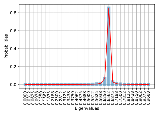
# >>> The phase is 0.6562 with probability 0.8516

qpe.result is the most probable ancilla outcome divided by \(2^{n_\mathrm{ancilla}}\). It is therefore restricted to a grid with spacing \(2^{-n_\mathrm{ancilla}}\), while qpe.result_probability is the probability assigned to that grid point.

For an ideal, isolated eigenphase, estimate_phase can fit the squared Dirichlet kernel to the complete QPE distribution and estimate the peak between adjacent grid points. This fit does not remove finite-shot uncertainty, noise, Trotter error, or errors caused by imperfect overlap with the target eigenstate. The phase is also periodic, so fits close to the 0/1 boundary require particular care.

fit_range can restrict the fit to an interval in which the phase is expected. If fit_range=None, the entire histogram is used and its centroid supplies the initial guess.

# Restrict the fit when an approximate phase range is known, for example:
# fit_range = (0.5, 0.7)
# Use the complete histogram when no suitable range is known.
fit_range = None

phi_estim = qpe.estimate_phase(fit_range=fit_range, verbose=True)
print("The deviation from the true phase is: ", np.abs(phi_estim - eigs[-1]))
# >>> Fit range: (0, 1)
# >>> The estimated phase using the Dirichlet kernel is: 0.6494081778695611
# >>> The deviation from the true phase is:  2.1647961090383034e-05

The sampled distribution and the fitted squared Dirichlet kernel can be plotted together:

# Plot the distribution.
fig, ax = qpe.plot(return_fig=True)
ax.plot(
    qpe.freqs,
    dirichlet_kernel_squared(qpe.freqs, phi_estim, 2**n_ancilla),
    "r",
    label="Dirichlet kernel squared",
)

Note

Increasing the number of ancilla qubits reduces the phase-bin spacing exponentially, but the controlled-unitary ladder uses \(2^{n_\mathrm{ancilla}}-1\) applications of \(U\). Accurate estimation also requires substantial overlap between the prepared state and the target eigenstate. If the input is a superposition of eigenstates, the measured distribution contains a corresponding mixture of eigenphases.

Density of States Quantum Phase Estimation (DOS-QPE)

Density of States Quantum Phase Estimation (DOS-QPE) applies phase estimation to a mixed probe state rather than to one prepared eigenstate. The resulting phase distribution approximates the density of eigenphases of the supplied unitary, weighted by the probe state. For a maximally mixed probe, each eigenstate contributes equally, so repeated eigenphases appear with weight proportional to their degeneracy. The method is described in arXiv:2510.14744.

OpenQARP prepares the mixed probe by adding a purification register with the same width as the system register. The system and purification registers are entangled with pairwise CNOT gates, and only the phase-estimation ancillas are measured. If hamming_weight=None, Hadamard gates prepare a maximally mixed probe over the full Hilbert space. If a Hamming weight is supplied, a Dicke-state purification restricts the probe to that fixed-particle-number subspace.

The complete circuit uses three registers:

• \(n_\mathrm{ancilla}\) phase-estimation qubits;

• \(n_\mathrm{qubits}\) system qubits on which the controlled unitary acts; and

• \(n_\mathrm{qubits}\) purification qubits that are not measured.

As in ordinary QPE, DOS-QPE estimates phases \(\phi\) defined by \(U|\psi\rangle=e^{2\pi i\phi}|\psi\rangle\). For \(U=e^{-iHt}\), energies map to \(\phi=(-Et/2\pi)\bmod 1\); DOS-QPE does not automatically undo the sign, time scaling, or phase wrapping.

Warning

The supplied unitary must be phase-exact. A global synthesis error becomes an observable shift when the unitary is controlled and therefore shifts every recovered eigenphase.

Note

The DOSQPEBlock documentation shows how to construct the underlying circuit directly.

Example: Fermi-Hubbard spectrum

from qarp.blocks import TrotterBlock
from qarp.operators import JordanWigner
from qarp.operators.models import fermi_hubbard
from qarp.algorithms import (
    DOSQPE,
    find_occupation_numbers,
    find_unique_eigs_and_occupation_numbers,
)
from qarp.algorithms import SpectrumEstimator
from qarp.endianness import bits_to_label
from qarp.engines import QarpEngine
from qarp.operators import FullyCommuting
from qarp.operators.functions import eigenspectrum

import numpy as np

# DOS-QPE parameters
n_qubits = 4
n_ancilla = 5

# Trotterization parameters
time = 2 * np.pi
n_trotter_steps = 4
trotter_order = 2
grouping = FullyCommuting()

# Use None for the full Hilbert space, or an integer for a fixed-Hamming-weight sector.
hamming_weight = None

qham = JordanWigner().encode_operator(fermi_hubbard((2,), t=0.14, U=0.231))
eigs = eigenspectrum(qham)
if eigs[0] < 0:
    # Shift the spectrum to be nonnegative. For this model it then lies in [0, 1).
    qham = qham + abs(eigs[0]) + np.finfo(float).eps
eigs = eigenspectrum(qham)
assert eigs[0] >= 0 and eigs[-1] < 1

# TrotterBlock implements exp(-iHt). Negating H gives exp(+iHt), so with
# time=2*pi, the DOS-QPE phases equal the shifted energies modulo 1.
circ_unitary = TrotterBlock(
    operator=-qham,
    n_qubits=n_qubits,
    steps=n_trotter_steps,
    time=time,
    order=trotter_order,
    grouping=grouping,
).build()

dosqpe = DOSQPE(
    unitary=circ_unitary,
    n_ancilla=n_ancilla,
    hamming_weight=hamming_weight,
    engine=QarpEngine(n_shots=10_000, seed=0),
).build()

run() returns the ancilla probability distribution. Its tuple keys are LSB-first, so bits_to_label converts them to the corresponding integer phase bins. Printing only the most probable bins is usually more useful than printing the complete \(2^{n_\mathrm{ancilla}}\)-entry dictionary.

distribution = dosqpe.run()
top_bins = sorted(
    (
        (bits_to_label(bits) / 2**n_ancilla, probability)
        for bits, probability in distribution.items()
    ),
    key=lambda item: item[1],
    reverse=True,
)[:5]
print([(round(phase, 5), round(probability, 4)) for phase, probability in top_bins])
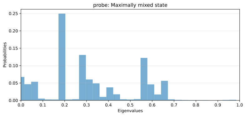
# >>> [(0.1875, 0.2495), (0.28125, 0.1307), (0.5625, 0.1221),
# >>>  (0.0, 0.0674), (0.3125, 0.0602)]

The finite ancilla register broadens an off-grid eigenphase across nearby bins. Degenerate eigenphases contribute proportionally more probability, which is why the fourfold-degenerate phase near 0.1874 produces the dominant peak.

# Plot the sampled phase distribution.
dosqpe.plot()

Increasing the number of ancilla qubits reduces the phase-bin spacing, but also increases the controlled-unitary ladder exponentially. More ancillas do not remove sampling noise, Trotter error, or phase wrapping.

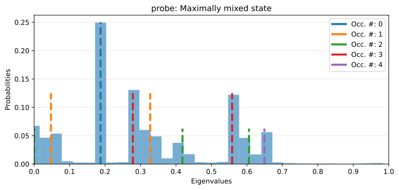
For validation, the sampled distribution can be compared with the exact spectrum. The following helper functions collect degenerate energies and label them by occupation number:

# Evaluate occupation numbers for the exact eigenstates.
occ_numbers = find_occupation_numbers(qham, n_qubits)

degeneracy_dict, unique_occ_numbers = find_unique_eigs_and_occupation_numbers(
    eigs,
    occ_numbers,
)
unique_eigs = np.array(list(degeneracy_dict))
degeneracies = np.array(list(degeneracy_dict.values()), dtype=float)
normalized_degeneracies = degeneracies / degeneracies.sum()

dosqpe.plot_against_spectrum(
    unique_eigs,
    normalized_degeneracies,
    unique_occ_numbers,
)

Spectrum estimation

SpectrumEstimator models the measured distribution as a line spectrum convolved with the QPE kernel. It can estimate off-grid eigenphases and their degeneracies, but it cannot recover spectral detail that is absent from the sampled data. Its accuracy remains limited by shot noise, circuit error, phase aliasing, and the number and separation of spectral lines relative to the ancilla resolution.

The dependency-light "esprit" mode performs parametric off-grid estimation. The "l2", "l1", "l2_adaptive", "l2_relaxed", and "atomic_norm" modes use convex optimization and require the [convex-optim] extra. The default "auto" mode evaluates the available candidate estimators and selects the reconstruction with the best data-fit score.

estimator = SpectrumEstimator(
    n_qubits=n_qubits,
    n_ancilla=n_ancilla,
    hamming_weight=hamming_weight,
    mode="esprit",
)
estimated_phases, estimated_degeneracies = estimator.estimate(
    distribution,
    freqs=dosqpe.freqs,
    integer_degeneracies=True,
)

print(np.round(estimated_phases, 4))
print(estimated_degeneracies)
# >>> [0.0626 0.188  0.2809 0.3194 0.401  0.5516 0.5681 0.6582 0.9975]
# >>> [1 4 2 2 1 1 2 1 2]

estimator.plot(
    distribution=distribution,
    freqs=dosqpe.freqs,
    true_phases=unique_eigs,
    true_degeneracies=degeneracies,
)

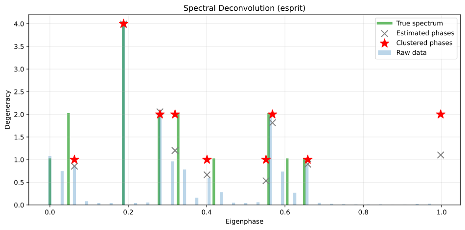
Here the estimator correctly identifies the dominant fourfold-degenerate line, but some nearby or weak lines are shifted, split, or merged. This is expected for a dense nine-line spectrum reconstructed from only 32 noisy phase bins; fitted output should not be treated as an exact eigenspectrum.

Multi-modal Multi-level Quantum Complex Exponential Least Squares (MMQCELS)

MMQCELS estimates several eigenvalues of a Hamiltonian simultaneously from the complex time-domain signal

\[Z(t) = \langle \Psi|e^{-iHt}|\Psi\rangle = \sum_k p_k e^{-i\lambda_k t}.\]

It fits the \(K\) dominant components by minimizing

\[\mathcal{L}(r, \theta) = \frac{1}{N}\sum_{n=1}^{N} \left|Z(t_n) - \sum_{k=1}^{K} r_k e^{-i\theta_k t_n}\right|^2.\]

The implementation follows Algorithm 2 of Ding and Lin, Quantum 7, 1136 (2023). At level \(j\), it draws independent times from the truncated Gaussian in Eq. (3), supported on \([-\gamma T_j,\gamma T_j]\), with \(T_j=2^jT_0\). Complex amplitudes are eliminated with linear least squares, leaving only the eigenvalues in the nonlinear optimization.

Only eigenstates with nonzero trial-state weight contribute to \(Z(t)\). Consequently, n_dominant_eigenvalues selects the number of dominant signal components, not necessarily the lowest \(K\) eigenvalues of the full Hamiltonian. Initial eigenvalue guesses must lie inside [lam_min, lam_max], which defaults to \([-\pi,\pi]\). The level fit is a bounded search over that interval, so optimizer (default ScipyOptimizer("L-BFGS-B")) must honour minimize(bounds=...): an optimizer whose supports_bounds is False (the gradient-descent family, Rotosolve) is refused with TypeError at construction rather than after the dataset is generated (see Optimizers).

Execution modes

execution_mode is required:

• "classical" diagonalizes a dense matrix or QubitOperator once.

• "statevector" evaluates a symbolic-time TrotterBlock exactly.

• "hadamard" evaluates both real and imaginary Hadamard-test quadratures.

In Hadamard mode, n_shots=None means one shot per quadrature, an integer requests finite sampling, and qarp.EXACT evaluates the infinite-shot protocol. n_shots is rejected in the other modes rather than silently ignored.

Parameter modes

Mode	Required schedule inputs	Meaning
standard (default)	T0, N0, Nj, and exactly one of n_levels or q	Paper schedule. With q, the class computes \(l=\max\{\lceil\log_2(q/(\epsilon T_0))\rceil,1\}\) and evaluates \(j=0,\ldots,l\), that is, l + 1 levels.
error_rate	T0; counts and level count may be overridden	Opt-in compatibility preset. It uses \(J=\lceil\log_2(1/\epsilon)\rceil+1\) from the predecessor single-mode QCELS paper, Nj=round(1/sqrt(epsilon)), and N0=max(Nj//2, 1). For a sequence-valued Nj, its first entry is used to derive N0. The count formula is a historical OpenQARP heuristic, not MM-QCELS Theorem 1.

T0 is always required because epsilon alone cannot determine a dimensionful initial time scale. All schedule values are validated when the class is constructed; missing, conflicting, non-finite, non-integral, or mode-incompatible inputs raise before circuits or optimizer state are built. Every evaluated level must use more samples than the requested number of dominant modes. In standard mode with an explicit n_levels, error_rate does not alter the schedule; it is used only by the q-derived schedule or by parameter_mode="error_rate".

Following QPE’s output convention, run() returns the sorted eigenvalue array and stores the same array in result and eigenvalues. Fitted amplitudes and run diagnostics remain available through amplitudes, level_losses, sample_counts, sampled_max_times, sampled_total_times, and optimizer_failed_starts. The latter counts discarded optimizer starts at each level; a level for which every start fails raises instead. n_initial_guesses counts all level-zero starts, including initial_eigenvalues when supplied.

Here is a minimal standard-mode setup using the versioned H2 molecular- integral snapshot. Run it from the repository root. See examples/algorithms/composite/mwe_mmqcels.ipynb for checked classical, StateVector, Hadamard, and error-rate-derived runs.

from pathlib import Path

import numpy as np

from qarp.algorithms import MMQCELS
from qarp.blocks import ComputationalBasisStateBlock
from qarp.operators import JordanWigner
from qarp.operators.integrals import restricted_integrals_to_fermion_operator
from qarp.operators.onv import onv_from_spatial_occupations

asset = Path("tests/assets/molecules/h2_0.735_sto3g.npz")
with np.load(asset) as data:
    fermion_operator = restricted_integrals_to_fermion_operator(
        float(data["constant"]), data["one_electron"], data["two_electron"]
    )

mapping = JordanWigner()
qham = mapping.encode_operator(fermion_operator)
onv = onv_from_spatial_occupations([2, 0])
state = ComputationalBasisStateBlock(mapping.encode_state(onv)).build()

algorithm = MMQCELS(
    operator=qham,
    state=state,
    execution_mode="classical",
    T0=1.25,
    N0=120,
    Nj=80,
    n_levels=5,
    n_dominant_eigenvalues=2,
    initial_eigenvalues=[-1.0, 0.5],
    seed=1,
    verbose=False,
)
eigenvalues = algorithm.run()
print(eigenvalues, algorithm.amplitudes)

Quantum Multiple Eigenvalue Gaussian filtered Search (QMEGS)

QMEGS (Quantum Multiple Eigenvalue Gaussian-filtered Search) estimates several eigenvalues of a Hamiltonian from a trial state and a time-evolution block. It samples the expectation value

\[Z(t) = \langle \psi | e^{-iHt} | \psi \rangle = \sum_k p_k e^{-i\lambda_k t},\]

where \(p_k = |\langle \lambda_k | \psi \rangle|^2\). A filtered density function evaluates candidate eigenvalues and returns the strongest peaks. The implementation follows Quantum 8, 1487 (2024).

The target indices refer to the eigenvalues returned by numpy.linalg.eigh (ascending order). They are not inferred by QMEGS, so use get_overlaps to choose states with the largest trial-state weights. A necessary condition is:

\[p_{\min} = \min_{k\in D} p_k > p_{\mathrm{tail}} = \sum_{k\notin D}p_k.\]

If this condition fails, build() raises ValueError. Increasing T improves resolution but also increases the evolution time and, for circuit execution, the circuit depth. Decreasing eta increases the internally calculated sample count.

Basic Usage:

The following example demonstrates QMEGS on a simple 2-qubit Hamiltonian:

import numpy as np
import qarp
from qarp.algorithms import get_overlaps
from qarp.algorithms import QMEGS
from qarp.blocks import SimpleBlock, SynthesizedTimeEvolutionBlock
from qarp.operators import QubitOperator
from qarp.operators.functions import eigenspectrum

np.random.seed(0)

# Define a 2-qubit Hamiltonian
hamiltonian = (
    QubitOperator("Z0 X1") + QubitOperator("Y0 Y1") + QubitOperator("X0 X1")
) * 0.25

n_qubits = 2

# Create trial state: |0⟩ ⊗ |+⟩
trial_state = SimpleBlock(n_qubits, name="trial_state")
trial_state.h(1)
trial_state.build()

overlaps, eigenvalues = get_overlaps(
    trial_state, hamiltonian, return_eigenvalues=True
)
# Select target eigenvalue indices (two with highest overlap)
sorted_indices = np.argsort(overlaps)[::-1]
target_indices = sorted_indices[:2].tolist()

unitary_block = SynthesizedTimeEvolutionBlock(
    n_qubits=n_qubits,
    operator=hamiltonian,
)

qmegs = QMEGS(
    unitary=unitary_block,
    state=trial_state,
    n_shots=qarp.EXACT,        # Exact analytical signal.
    target_indices=target_indices,
    sigma=1.0,
    eta=0.01,
    T=100,
    mode_dataset="analytical",
).build()

# Run and get estimated eigenvalues
result = qmegs.run()
print("Exact eigenvalues:", np.round(eigenspectrum(hamiltonian), 8))
print("Target indices:", target_indices)
print("Estimated eigenvalues:", np.round(sorted(result), 6))
print("Exact target eigenvalues:", np.round(sorted(eigenvalues[target_indices]), 6))
# >>> Estimated eigenvalues: [0.102785 0.60639]
# >>> Exact target eigenvalues: [0.103553 0.603553]

Using Trotter Time Evolution:

For Hamiltonians that require Trotterization, use TrotterBlock:

import qarp
from qarp.blocks import TrotterBlock

# Build Trotter unitary
trotter_unitary = TrotterBlock(
    n_qubits=n_qubits,
    operator=hamiltonian,
    steps=10,
    order=4,
)

# Create QMEGS
qmegs = QMEGS(
    unitary=trotter_unitary,
    state=trial_state,
    n_shots=qarp.EXACT,        # Use statevector simulation
    target_indices=target_indices,
    sigma=1.0,
    eta=0.01,
    T=100,
).build()

result = qmegs.run()

print("Estimated eigenvalues with Trotter:", sorted(result))

Note

Both TrotterBlock and SynthesizedTimeEvolutionBlock implement the standard \(\exp(-iHt)\) convention, so no sign adapter is needed on the QMEGS side.

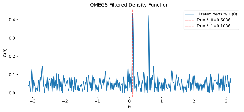
Visualizing the Filtered Density Function:

The filtered density function reveals peaks at eigenvalue locations:

import matplotlib.pyplot as plt

# Generate dataset and compute filtered density
qmegs.run()

J = int(np.floor(2 * np.pi * qmegs.T / qmegs.q))
theta_js = np.array([-np.pi + j * qmegs.q / qmegs.T for j in range(J + 1)])
G_js = qmegs.filtered_density_function(qmegs.dataset, theta_js, qmegs.n_samples)

# Plot with true eigenvalue markers
plt.figure(figsize=(10, 4))
plt.plot(theta_js, G_js, label='Filtered density G(θ)')
for i, eig in enumerate(eigenvalues[target_indices]):
    plt.axvline(x=eig, color='r', linestyle='--', alpha=0.7,
                label=f'True λ_{i}={eig:.4f}')
plt.xlabel('θ')
plt.ylabel('G(θ)')
plt.title('QMEGS Filtered Density Function')
plt.legend()
plt.show()

Sampling Mode:

To use shot-based circuit measurements, select mode_dataset="sampling" and pass a sampling primitive and a compatible engine:

Where ``p_min`` / ``p_tail`` come from: the algorithm’s a-priori inputs (Theorem 1) are produced by overlaps="classical" (the default) — an \(O(4^n)\) diagonalisation of the Hamiltonian plus one exact trial statevector read through the engine. That is a classical validation step and is refused with CapabilityError on a noisy or routed engine. Pass overlaps=(pmin, ptail) to supply the two numbers yourself: no spectrum is computed, the sampling path runs on any engine, and only len(target_indices) (the number of eigenvalues to extract) is consulted. mode_dataset="analytical" synthesises the signal from the spectrum and therefore requires overlaps="classical".

from qarp.engines import QarpEngine
from qarp.algorithms import HadamardTest

# Create engine and primitive for measurements
engine = QarpEngine()
primitive = HadamardTest()

qmegs = QMEGS(
    unitary=unitary_block,
    state=trial_state,
    n_shots=10000,
    target_indices=target_indices,
    mode_dataset="sampling",
    mode_time="rvs",
    engine=engine,
    primitive=primitive,
).build()

result = qmegs.run()

print("Estimated eigenvalues with sampling:", sorted(result))

The default StateVector primitive is exact, even in sampling mode. Use HadamardTest to model finite-shot measurements. A real device engine must support the same primitive and time-dependent unitary block.

Algorithm Parameters:

• sigma (float): Truncation level for Gaussian filtering. Smaller values concentrate sampling near t=0. Default: 1.0

• eta (float): Error tolerance controlling the number of samples. Smaller values require more samples but improve accuracy. Default: 0.01

• T (int): Time window for sampling. Larger values provide better eigenvalue resolution but require more circuit depth. Default: 100

• mode_dataset (str): 'analytical' computes the signal from the eigendecomposition; 'sampling' executes one circuit per sampled time

• mode_time (str): Time sampling method - 'rvs' for fast scipy sampling or 'rejection_sampling' for custom filtering functions

• filtering_function (callable): Custom acceptance density for mode_time='rejection_sampling'. Defaults to the truncated Gaussian density

Custom Filtering Functions:

You can provide a custom filtering function for advanced use cases:

import qarp

def custom_filter(t, sigma, T):
    """Custom filtering function."""
    return np.exp(-T * t**2 / 2) * (1 + 0.1 * np.cos(t))

qmegs = QMEGS(
    unitary=unitary_block,
    state=trial_state,
    n_shots=qarp.EXACT,
    target_indices=target_indices,
    filtering_function=custom_filter,
    mode_time='rejection_sampling',  # Required for custom functions
).build()

result = qmegs.run()

# A custom filter changes the time distribution and may reduce accuracy.
print("Estimated eigenvalues with custom filter:", sorted(result))

Performance Considerations:

The number of samples required scales as:

\[N_{\text{samples}} = \mathcal{O}\left( \frac{\log((T/q + |D|)/\eta)}{(p_{\min}-p_{\mathrm{tail}})^2} \right)\]

where \(D\) is the selected target-index set. For high precision, the sample count can become large and long-time Trotter or hardware errors can dominate.

Note

QMEGS is most effective when the trial state has good overlap with the target eigenstates (\(p_{\min}\) large) and minimal overlap with non-target eigenstates (\(p_{\text{tail}}\) small). Constructing good trial states often requires problem-specific knowledge or preliminary variational optimization.

Shor factoring and quantum order finding

The Shor composite algorithm factors a small composite integer by combining quantum multiplicative-order finding with classical continued fractions and greatest-common-divisor calculations. For a base \(a\) coprime to the number \(N\), the quantum circuit samples phases associated with the periodic function

\[f(x) = a^x \bmod N.\]

The period \(r\) is accepted only after the classical check \(a^r \bmod N = 1\). When \(r\) is even and \(a^{r/2} \not\equiv \pm 1 \pmod N\), the factors follow from \(\gcd(a^{r/2}-1,N)\) and \(\gcd(a^{r/2}+1,N)\).

OpenQARP exposes the two reusable quantum blocks behind this workflow:

• ModularMultiplicationBlock(m, N) implements the complete LSB-indexed basis permutation \(|x\rangle\mapsto|mx\bmod N\rangle\) for \(x<N\) and fixes every basis label \(x\geq N\).

• OrderFindingBlock(a, N) prepares a counting register and a work register, applies controlled modular powers, and finishes with an inverse QFT. It contains no measurement commands; Sampler measures and marginalises the counting qubits.

The following deterministic reference calculation factors 15. Eight counting qubits give phase bins at 0, 64, 128, and 192 for the order \(\operatorname{ord}_{15}(2)=4\). force_quantum=True guarantees that the circuit is executed (see below).

import qarp
from qarp.algorithms import Sampler
from qarp.algorithms import Shor
from qarp.endianness import bits_to_label

shor = Shor(
    15,
    base=2,
    force_quantum=True,
    primitive=Sampler(n_shots=qarp.EXACT),
).build()

factors = shor.run()
peaks = sorted(
    (bits_to_label(bits), round(probability, 4))
    for bits, probability in shor.distributions[2].items()
    if probability > 1e-10
)

print("order:", shor.orders[2])
print("phase bins:", peaks)
print("factors:", factors)
# >>> order: 4
# >>> phase bins: [(0, 0.25), (64, 0.25), (128, 0.25), (192, 0.25)]
# >>> factors: (3, 5)

Sampler tuples are LSB-first. Use bits_to_label to convert a tuple to the integer phase label; the corresponding normalized phase is that label divided by \(2^t\), where \(t\) is the number of counting qubits. With finite shots, an attempt may not observe enough useful peaks and run() may therefore return None. Multiple configured bases are executed as one batch, and inconclusive attempts do not prevent a later base from succeeding.

Bases are processed in attempt order, as in Shor’s sequential algorithm. In the default mode every coprime base gets an order-finding circuit, and the first non-coprime base ends the attempt list with \(\gcd(a, N)\) as a classical fallback that run() returns only when every quantum attempt was inconclusive. Because small moduli have many non-coprime bases, a default call on \(N=15\) frequently ends at that fallback. force_quantum=True disables the shortcut: random bases are drawn coprime, a supplied non-coprime base is rejected, and even or perfect-power inputs raise because they lie outside the preconditions of Shor’s order-finding theorem.

build() prepares the samplers and never factors; every classical exit happens in run(). Prime inputs are rejected at build(). Even integers and exact perfect powers are factored classically without a circuit in the default mode. The return value is one sorted non-trivial factor pair; it is not a recursive prime factorization.

Warning

This first implementation is an exact small-integer reference, not a scalable implementation of Shor’s algorithm. Modular multiplication is synthesized by enumerating computational-basis permutations, has exponential gate cost, and is limited to six work qubits, so Shor accepts \(N \le 64\) at construction. Exact sampling of the order- finding circuit takes about 2 s at that limit and would take 31 s one work qubit beyond it. It must not be used to make cryptographic-scale or asymptotic-speedup claims.

The mathematical workflow follows Shor’s original factoring and order-finding construction in SIAM Journal on Computing 26, 1484–1509 (preprint). A future scalable arithmetic backend may use a polynomial reversible construction such as Beauregard’s 2n+3-qubit circuit while retaining the public OpenQARP block and algorithm interfaces described here.

Variational Quantum Eigensolver (VQE)

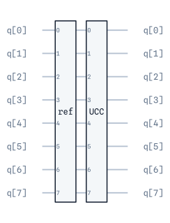
One of the most popular VQE approaches is the Unitary Coupled Cluster (UCC) method and its variants. It relies on a basis generation by means of excitation operators acting on a chosen reference state. Every excitation operator involved is related to a variational parameter which is optimized by minimization of the energy surface spanned by the Hamiltonian of the system and the trial circuit generated.

The UCC quantum circuit is of the form

\[|\psi\rangle = \sum_k e^{i \theta_k \hat{A}_k} |\rm{ref}\rangle,\]

where \(\hat{A}_k\) are the chosen excitation operators with corresponding variational parameters \(\theta_k\). The different choices of operators make the difference in the UCC variants. A common choice is to use all the singles and doubles operators, \(a_i^+ a_j\) and \(a_i^+ a_j^+ a_l a_k\), respectively. Other considerations to reduce this number of operators, for example based on symmetries of the system, are encouraged as they scale as \(\mathcal{O}(N^2)\) and \(\mathcal{O}(N^4)\).

OpenQARP offers versatility when building an UCC object. First, let’s define the problem example we want to apply it to: We’ll choose an equally spaced H4 chain, loaded from its stored STO-3G integrals. Run the snippet from the repository root:

from pathlib import Path
import numpy as np

from qarp.operators import JordanWigner

from qarp.blocks import ComputationalBasisStateBlock, UCCBlock, CompositeBlock
from qarp.operators.integrals import restricted_integrals_to_fermion_operator

from qarp.algorithms import StateVector
from qarp.operators.onv import onv_from_spatial_occupations

asset = Path("tests/assets/molecules/h4_1.000_sto3g.npz")
with np.load(asset) as data:
    fop = restricted_integrals_to_fermion_operator(
        float(data["constant"]), data["one_electron"], data["two_electron"]
    )

onv = onv_from_spatial_occupations([2, 2, 0, 0])

qham = JordanWigner().encode_operator(fop)

ref = ComputationalBasisStateBlock(onv, name="ref")
ucc = UCCBlock(onv, singles=True, doubles=True)
ansatz = CompositeBlock([ref, ucc])
ansatz.build()
ansatz.plot()

This variational algorithm finds a set of optimal parameters minimizing the expectation value of the Hamiltonian in qubit operator form with the UCC ansatz as we have defined it with the excitation operators. Now we have everything to run the UCC-VQE calculation by using:

from qarp.algorithms import VQE
ansatz.build()

vqe = VQE(operator=qham, ket=ansatz, verbose=True, gradient=True, primitive=StateVector())
vqe.build()
e, p = vqe.run()

We observe that we have chosen the standard StateVector as our measurement strategy, but the OpenQARP user is not limited to this. We can run a noisy VQE simulation on a prescribed device with a certain architecture by specifying the appropriate measurement strategy. Note that most of the presented algorithms enable the usage of gradients by setting gradient=True in the constructor (the engine’s default method: adjoint backpropagation for StateVector, the batched parameter shift for sampled primitives), or to a method name such as gradient="parameter-shift" — see Gradients.

It is also possible to choose a different primitive to StateVector for these types of algorithm, provided they can calculate an expectation value. Be warned, however, that without some measurement reduction functionality these other primitives can be expensive to run for a full variational loop.

Projected Variational Quantum Eigensolver (Projected VQE)

ProjectedVQE implements variation after projection. For an ansatz \(|\psi(\boldsymbol{\theta})\rangle\), Hamiltonian \(H\), and symmetry projector \(P\), it minimizes the projected Rayleigh quotient

\[E_P(\boldsymbol{\theta}) = \frac{\langle P\psi(\boldsymbol{\theta})|H| P\psi(\boldsymbol{\theta})\rangle} {\langle P\psi(\boldsymbol{\theta})| P\psi(\boldsymbol{\theta})\rangle}.\]

This allows a parameterized circuit that does not preserve a symmetry to be optimized within a chosen sector. The operator must be a OpenQARP QubitOperator, and ket must be a built or buildable parameterized block on the same number of system qubits as the projector.

examples/algorithms/composite/mwe_projected_vqe.ipynb works this through on a two-site Fermi-Hubbard model whose global ground state lies outside the requested sector, so the projector is what makes the answer the right one.

projector accepts one block or a sequence of the projector blocks described in Projector Blocks. A sequence is converted to a matrix product; it represents the intersection of sectors when the projectors commute. For a custom projector, pass a dense projector_matrix in qarpx’s LSB basis ordering instead. projector and projector_matrix are mutually exclusive. If neither is supplied, the identity is used and the objective reduces to ordinary statevector VQE.

Projected VQE uses a specialized statevector objective. It simulates only the bare ansatz, converts known projector blocks to dense system-register matrices, and applies the projection by classical matrix multiplication during each objective evaluation. The LCU projector circuits and their ancillas are not simulated in the optimization loop. This is efficient for small statevector calculations, but it is not a finite-shot or hardware postselection workflow, and its objective is a ratio, so neither the adjoint nor the parameter-shift rule applies (gradient="finite-diff" does). The default optimizer is COBYLA.

If the squared norm of the projected state is below postselection_tol, the objective returns positive infinity. After run(), the normalized projected state and the unprojected ansatz state are available as final_projected_statevector and final_ansatz_statevector. run() returns (energy, parameters), while optimal_parameters provides the order-safe symbol-to-value mapping.

In this two-qubit example, the ansatz spans several particle-number sectors. Projection retains the one-particle sector, where \(H=(X_0X_1+Y_0Y_1)/2\) has exact ground energy \(-1\):

import numpy as np
from sympy import Symbol

from qarp.algorithms import ProjectedVQE
from qarp.blocks import ParticleNumberProjectorBlock, SimpleBlock
from qarp.operators import QubitOperator
from qarp.optimizers import ScipyOptimizer

theta = Symbol("theta")
ansatz = SimpleBlock(2, name="Ansatz")
ansatz.ry(0, theta)
ansatz.h(1)
ansatz.build()

hamiltonian = (
    0.5 * QubitOperator("X0 X1")
    + 0.5 * QubitOperator("Y0 Y1")
)
projector = ParticleNumberProjectorBlock(n_qubits=2, Npart=1)

projected_vqe = ProjectedVQE(
    operator=hamiltonian,
    ket=ansatz,
    projector=projector,
    initial_parameters=np.array([0.2]),
    optimizer=ScipyOptimizer(
        "COBYLA", options={"maxiter": 100, "tol": 1e-10}
    ),
).build()
energy, parameters = projected_vqe.run()

assert np.isclose(energy, -1.0, atol=1e-8)
assert np.allclose(
    projected_vqe.final_projected_statevector[[0, 3]], 0.0, atol=1e-10
)

ADAPT-VQE

ADAPT-VQE has become quite popular in the scientific community due to its capability to generate expressive ansatze within a small number of iterations. This algorithms builds wavefunctions of the form

\[|\psi\rangle = \prod_k e^{i \theta_k \hat{A}_k} |\rm{ref}\rangle,\]

where \(\hat{A}_k\) are the chosen excitation operators with corresponding variational parameters \(\theta_k\), obtained classically by minimizing the energy surface. ADAPT-VQE iteratively updates the reference state \(|\rm{ref}\rangle\) with an excitation operator having the largest energy gradient according to the formula

\[\frac{\partial E}{\partial \theta_k} = i \langle \psi |[H, \hat{A}_k]| \psi \rangle,\]

with \(H\) being the Hamiltonian of the system we want to solve. The algorithm will stop when all these gradients are below a certain threshold.

OpenQARP offers the possibility to build your ADAPT-VQE object with flexible options for the reference state, excitation operators, optimizers and iterations.

We illustrate the process taking as an example LiH in a (2e, 3o) active space, reduced from the stored LiH/STO-3G integrals. Run it from the repository root:

from pathlib import Path

import numpy as np

from qarp.operators import JordanWigner
from qarp.operators.integrals import (
    active_space_integrals,
    restricted_integrals_to_fermion_operator,
)
from qarp.operators.onv import onv_from_spatial_occupations
from qarp.operators.ucc import ucc_singles_and_doubles
from qarp.blocks import ComputationalBasisStateBlock
from qarp.algorithms import AdaptVQE, StateVector

asset = Path("tests/assets/molecules/lih_1.59_sto3g.npz")
with np.load(asset) as data:
    integrals = active_space_integrals(
        float(data["constant"]),
        data["one_electron"],
        data["two_electron"],
        n_electrons=int(data["nelectron"]),
        active_electrons=2,
        active_orbitals=3,
    )
fermion_operator = restricted_integrals_to_fermion_operator(*integrals)

mapping = JordanWigner()
qop = mapping.encode_operator(fermion_operator)
onv = onv_from_spatial_occupations([2, 0, 0])

fucc = ucc_singles_and_doubles(onv, generalised=False, spin_conserving=False)[0]
qucc = mapping.encode_operator(fucc)
print(onv)


ref = ComputationalBasisStateBlock(onv)
ref.build()

adapt = AdaptVQE(
    reference_block=ref,
    system_hamiltonian=qop,
    excitation_pool=qucc,
    primitive=StateVector(),
    gradient=True,
    gradient_thresh=1e-9,
    convergence_thresh=1e-10,
    exc_per_iter=1
)
adapt.build()
s0_en, _ = adapt.run()

After we build our ADAPT-VQE object, we may be interested in just running a few iterations in order to obtain an expressive ansatz to use in another quantum algorithm with minimal cost. We may use adapt.iterate() as times as needed to update the wavefunction.

If, on the other hand, we would like to run the full ADAPT-VQE algorithm, we may use adapt.run(max_iter=max_iter). The output will be the final energy, close to the ground-state energy of the Hamiltoinan within a threshold, and the optimal parameters. If you’d like to access the information on the parameters and excitation operators involved, you may do so by calling adapt.ansatz_parameters_dict and adapt.ansatz_excitations, respectively.

In addition to the original ADAPT-VQE method, the implementation in OpenQARP allows to add more than one term in an iteration, e.g. AdaptVQE(.., exc_per_iter = 5).

It is worth noting that if using some other primitive besides StateVector to evaluate the energies and commutators, a block must representing the Hamiltonian must also be passed in the operator_block argument. This is because for StateVector, it is clear how to handle the commutators, but for other primitives it is not, and it is up to the user to create a block which represents the operator.

Variational Quantum Deflation (VQD)

Variational Quantum Deflation (VQD) computes a sequence of approximate eigenstates with separate parameterized ansatz blocks. The first state minimizes the energy; each later state minimizes the energy plus penalties for overlap with the states already found.

For state \(k\), the objective is

\[\mathcal{L}_k = \langle \psi_k | H |\psi_k\rangle + \sum_{i=0}^{k-1} \beta_i |\langle \psi_i |\psi_k\rangle|^2,\]

where \(|\psi_k\rangle\) is the current ansatz and \(\beta_i\) are penalty weights. OpenQARP optimizes the kets sequentially, fixing each previously optimized ket before moving to the next one. The penalty weights discourage collapse into lower-energy states, but a finite ansatz and an unsuitable penalty can still produce mixtures or skip eigenstates.

The kets argument must contain one parameterized block for every state to optimize; bare state-preparation blocks with no symbols are rejected. weights must have exactly one entry fewer than kets. initial_parameters accepts one vector per ket, or a mapping from that ket’s symbols to values. The mapping form is order-independent and is preferred when symbols are constructed dynamically.

The default primitive is StateVector. gradient=True (or a method name, see Gradients) differentiates the energy and the deflation penalties — the overlap gradient is that of |⟨ψ_i|ψ⟩|² on every method. VQD.run() returns (energies, state_parameters), where the second item is a list of per-state symbol-to-value dictionaries. get_final_state_block(index) returns the corresponding ket with those parameters bound.

The following H₂ example optimizes four states. The first ket targets the ground state and the next three are deflated in sequence. It loads the stored H₂/STO-3G integrals, so run it from the repository root:

from pathlib import Path

import numpy as np

from qarp.blocks import UCCBlock, MappedONVStateBlock, CompositeBlock
from qarp.operators import JordanWigner
from qarp.operators.integrals import restricted_integrals_to_fermion_operator
from qarp.operators.onv import onv_from_spatial_occupations
from qarp.algorithms import VQD
from qarp.optimizers import ScipyOptimizer

np.random.seed(42)

asset = Path("tests/assets/molecules/h2_0.735_sto3g.npz")
with np.load(asset) as data:
    fermion_operator = restricted_integrals_to_fermion_operator(
        float(data["constant"]), data["one_electron"], data["two_electron"]
    )

mapping = JordanWigner()
qop = mapping.encode_operator(fermion_operator)
onv = onv_from_spatial_occupations([2, 0])

ucc = UCCBlock(onv, generalised=True)
ref = MappedONVStateBlock(onv)
wfn = CompositeBlock([ref, ucc]).build()

Now, we run the approach for different ket instances:

kets = [wfn.refresh_symbols(f"_{i}").build() for i in range(4)]

parameters = []
for k in kets:
    parameters.append(np.random.rand(len(k.symbols)))

vqd = VQD(
    operator=qop,
    kets=kets,
    weights=[5, 5, 5],
    initial_parameters=parameters,
    gradient=False,
    optimizer=ScipyOptimizer(method="COBYLA"),
    verbose=False,
)
vqd.build()
energies, state_parameters = vqd.run()
print("VQD energies:", np.round(np.real(energies), 6))
# >>> VQD energies: [-1.137306 -0.524616 -0.162753  0.495058]

The reported values are expectation energies, not penalty-function values. Their quality depends on the ansatz expressiveness, the initial parameters, and the penalty weights. Random initial parameters can help avoid staying in an unintended symmetry sector; for reproducibility, seed NumPy as in the example. The optimizer may return states in a different order or skip levels when the ansatz or penalties are inadequate.

Weighted Subspace-Search Variational Quantum Eigensolver (SS-VQE)

SS-VQE obtains several eigenstates in one optimization by applying a shared parameterized ansatz to a list of mutually orthogonal basis states. OpenQARP minimizes the weighted energy objective described by Fujii et al. in Physical Review Research 1, 033062:

\[\mathcal{L}_w (\boldsymbol{\theta}) = \sum_{i=0}^{k-1} w_i \langle \psi_i | U^\dagger(\boldsymbol{\theta}) H U(\boldsymbol{\theta}) | \psi_i \rangle.\]

Here \(|\psi_i\rangle\) are the supplied basis-state blocks and \(k\) is their number. The order of basis_state_blocks and weights is significant: the energy at index i corresponds to basis state i. To associate lower energies with the earlier states, choose weights in descending order. The weights and basis-state lists must have the same length, and the basis states should be distinct and mutually orthogonal. Applying the same unitary ansatz preserves their orthogonality.

The OpenQARP class is SSVQE. ansatz_block must be parameterized; initial_parameters may be a positional vector or a symbol-to-value mapping. The default primitive is StateVector and the default optimizer is conjugate gradient. gradient=True or a method name (see Gradients) differentiates the weighted objective on any scalar primitive. run() returns (energies, parameters), where energies is in basis-state order. get_final_state_block(index) returns the optimized ansatz applied to the selected basis state.

The following H₂ example uses four basis states and a descending weight schedule. It loads the stored H₂/STO-3G integrals, so run it from the repository root:

from pathlib import Path

import numpy as np

from qarp.operators import JordanWigner
from qarp.operators.integrals import restricted_integrals_to_fermion_operator
from qarp.operators.onv import onv_from_spatial_occupations
from qarp.blocks import ComputationalBasisStateBlock, UCCBlock
from qarp.algorithms import SSVQE

np.random.seed(0)

asset = Path("tests/assets/molecules/h2_0.735_sto3g.npz")
with np.load(asset) as data:
    fermion_operator = restricted_integrals_to_fermion_operator(
        float(data["constant"]), data["one_electron"], data["two_electron"]
    )

mapping = JordanWigner()
qop = mapping.encode_operator(fermion_operator)
onv = onv_from_spatial_occupations([2, 0])

ansatz = UCCBlock(occupation_number_vector=onv, generalised=True).build()
basis_states = [
    ComputationalBasisStateBlock([1, 1, 0, 0]).build(),
    ComputationalBasisStateBlock([0, 1, 1, 0]).build(),
    ComputationalBasisStateBlock([0, 0, 1, 1]).build(),
    ComputationalBasisStateBlock([1, 0, 0, 1]).build(),
]
initial_parameters = np.random.rand(len(ansatz.symbols))

ssvqe = SSVQE(
    operator=qop,
    ansatz_block=ansatz,
    basis_state_blocks=basis_states,
    weights=[12, 6, 3, 1],
    initial_parameters=initial_parameters,
    verbose=False,
)
ssvqe.build()
energies, parameters = ssvqe.run()
print("SS-VQE energies:", np.round(np.real(energies), 6))
# >>> SS-VQE energies: [-1.137306 -0.524616  0.495058 -0.162753]

The values are expectation energies, not the weighted objective value. Their order follows basis_state_blocks (and is therefore not necessarily sorted by energy). Random initial parameters can help avoid an unintended symmetry sector; seed NumPy when reproducibility is important. With a finite-shot primitive the parameter-shift gradient is shot-noisy; prefer a gradient-free optimizer or n_shots=qarp.EXACT.

ADAPT-VQD

ADAPT-VQD adaptively constructs an ansatz for an excited state while penalizing overlap with one or more previously optimized states. At each iteration it scans an excitation pool, adds the operators with the largest gradients, and optimizes the resulting ansatz. The objective is

\[\mathcal{L}(\theta) = \langle\psi(\theta)|H|\psi(\theta)\rangle + \sum_i \beta_i |\langle\phi_i|\psi(\theta)\rangle|^2,\]

where orthogonal_states supplies the \(|\phi_i\rangle\) and betas supplies the corresponding penalty coefficients. The two lists must have the same length, and the orthogonal-state blocks should already be optimized and built. The implementation follows Phys. Chem. Chem. Phys. (2021) 23 (46): 26438–26450.

term_gradient="ADAPT-VQD" (the default) includes the deflation penalties when ranking pool operators. Set term_gradient="ADAPT-VQE" to rank operators with the unpenalized ADAPT-VQE gradient while retaining the VQD objective during optimization. exc_per_iter controls how many operators are added per iteration; diminishing=True removes selected operators from the pool. gradient_thresh stops pool selection when the largest gradient falls below the threshold. run(max_iter=...) returns (final_energy, parameters).

The usual workflow is to obtain a ground-state block first, then pass it in orthogonal_states when constructing AdaptVQD. The example again uses LiH in a (2e, 3o) active space and runs from the repository root:

from pathlib import Path

import numpy as np

from qarp.blocks import MappedONVStateBlock
from qarp.operators import JordanWigner
from qarp.operators.integrals import (
    active_space_integrals,
    restricted_integrals_to_fermion_operator,
)
from qarp.operators.onv import onv_from_spatial_occupations
from qarp.operators.ucc import ucc_singles_and_doubles
from qarp.optimizers import ScipyOptimizer
from qarp.algorithms import AdaptVQD, AdaptVQE

asset = Path("tests/assets/molecules/lih_1.59_sto3g.npz")
with np.load(asset) as data:
    integrals = active_space_integrals(
        float(data["constant"]),
        data["one_electron"],
        data["two_electron"],
        n_electrons=int(data["nelectron"]),
        active_electrons=2,
        active_orbitals=3,
    )
fermion_operator = restricted_integrals_to_fermion_operator(*integrals)

mapping = JordanWigner()
qop = mapping.encode_operator(fermion_operator)
onv = onv_from_spatial_occupations([2, 0, 0])
fucc = ucc_singles_and_doubles(onv, generalised=False, spin_conserving=False)[0]
qucc = mapping.encode_operator(fucc)

# First optimize the ground state.
adapt = AdaptVQE(
    reference_block=MappedONVStateBlock(onv).build(),
    system_hamiltonian=qop,
    excitation_pool=qucc,
    optimizer=ScipyOptimizer("BFGS"),
    diminishing=False,
    verbose=False,
    gradient=False,
    exc_per_iter=2,
)
adapt.gradient_thresh = 1e-4
adapt.build()
s0_en, _ = adapt.run()

ground_state = adapt.get_final_state_block()
adaptvqd = AdaptVQD(
    reference_block=MappedONVStateBlock(onv).build(),
    hamiltonian=qop,
    excitation_pool=qucc,
    orthogonal_states=[ground_state],
    betas=[1.0],
    optimizer=ScipyOptimizer("BFGS"),
    diminishing=False,
    verbose=False,
    gradient=False,
)
adaptvqd.gradient_thresh = 1e-4
adaptvqd.terminate_if_coeff_zero=True
adaptvqd.build()
s1_en, _ = adaptvqd.run()
print("Ground-state energy:", round(float(s0_en), 6))
print("ADAPT-VQD energy:", round(float(s1_en.real), 6))
# >>> Ground-state energy: -7.863228
# >>> ADAPT-VQD energy: -7.721646

The AdaptVQD hamiltonian must be a OpenQARP QubitOperator and the excitation pool must contain QubitOperators acting on the same qubits as reference_block. Use get_final_state_block() after run() to obtain the optimized, parameter-bound excited-state block. The returned energy is the expectation value \(\langle\psi|H|\psi\rangle\), not the penalized objective. For noisy primitives, use a gradient-free optimizer unless reliable analytic gradients are available; pool and optimization thresholds may need retuning for shot noise.

Quantum Approximate Optimization Algorithm (QAOA)

The Quantum Approximate Optimization Algorithm (QAOA) is a variational quantum algorithm designed to solve graph-based combinatorial optimization problems, such as Max-Cut. It consists of \(p\) layers, where each layer sequentially applies a cost operator and a mixer operator. The cost operator encodes the Hamiltonian formulation of the optimization problem.

The QAOA wavefunction is defined as:

\[|\psi_p\rangle = U_M(B, \beta_p) U_P(C, \gamma_p) \dots U_M(B, \beta_1) U_P(C, \gamma_1) |s\rangle\]

The circuit symbols are gamma_<layer> and beta_<layer> (ASCII, so to_qasm3() is valid OpenQASM 3). block.symbols is sorted by name, so it reads (beta_0, …, gamma_0, …) rather than the per-layer (gamma, beta) order other SDKs use positionally — pass initial_parameters as a {symbol: value} mapping, or go through parameter_map, rather than zipping a vector.

where:

• \(U_P(C, \gamma) = e^{-i\gamma C}\) is the phase separator, applying a phase shift based on the cost Hamiltonian \(C\).

• \(U_M(B, \beta) = e^{-i\beta B}\) is the mixer, evolving the state under the mixing Hamiltonian \(B\).

• \(|s\rangle\) is the initial state, typically an equal superposition of all computational basis states.

The parameters \(\gamma\) and \(\beta\) are optimized classically to minimize the expectation value of the cost function. Therefore, the total number of parameters to optimize is \(2p\).

An example of the pipeline for using QAOA to solve a Max-Cut problem is as follows:

1. Create a Graph

We begin by creating a simple weighted graph with 4 nodes and 2 edges:

from qarp.graphs import Graph

graph = Graph()
graph.add_edges_from([(0, 1, {"weight": 2.0}), (2, 3, {"weight": 2.0})])

2. Initialize the QAOA Object

Next, we initialize and build the QAOA object. While several parameters can be tuned, we use default values for simplicity:

from qarp.algorithms import QAOA

n_layers = 2
qaoa = QAOA(graph, n_layers=n_layers, verbose=True, initial_parameters=[.1] * 2 * n_layers).build()
fun, x = qaoa.run()

OpenQARP also supports Hamiltonian-based formulations with linear and quadratic terms. The following example penalizes specific solutions by adding linear terms:

from qarp.operators import QubitOperator

ham = QubitOperator("Z0 Z1") + QubitOperator("Z1 Z2")
ham += QubitOperator("Z0")  # penalize (0, 1, 0)

qaoa = QAOA(ham, n_layers=4, verbose=True, gradient=False).build()
fun, x = qaoa.run()

3. Analyze the Solutions

After running QAOA, we obtain the optimal parameters and minimum cost. To extract solutions, we apply the parameters to the wavefunction and sample it. The most probable bitstrings correspond to optimal solutions.

The following code snippet demonstrates how to sample the ansatz and extract the most probable solution:

from qarp.engines import QarpEngine
from qarp.algorithms import Sampler

bound = qaoa.get_final_state_block()  # result.x already bound in sorted-symbol order (§17)

sampler = Sampler(ket=bound, n_shots=10_000)
engine = QarpEngine()
engine.build([sampler])
counts = engine.run({})[0]
total = sum(counts.values())
probs = {k: v / total for k, v in counts.items()}

from qarp.plotting import plot_histogram
plot_histogram(probs, show_all_solutions=True, return_plotter=False)

For a more detailed pipeline, refer to the minimal working examples in the /examples/ directory.

Pauli Correlation Encoding Algorithm (PCE)

The Pauli Correlation Encoding (PCE) algorithm is another variational quantum approach for solving graph-based optimization problems such as Max-Cut. Unlike QAOA, PCE uses a problem-independent ansatz. In this example, we use the HEABlock provided by OpenQARP. Additionally, PCE allows multiple graph nodes to be encoded per qubit: on \(n\) qubits an order-\(k\) encoding supplies \(3\binom{n}{k}\) Pauli correlators, and so encodes that many nodes — \(3n(n-1)/2\) in the common \(k = 2\) case. calculate_qubits inverts this, returning the smallest \(n\) that fits the node count. Notably, the algorithm’s complexity is independent of the graph’s edge density.

Note that, in the original paper they propose PCE for solving MaxCut-like problems. In this implementation we have extended its functionality to overcome this limitation. This can be tuned by changing classical_function and quantum_function in the arguments of the constructor of the algorithm.

Let’s check an example of a MaxCut-like problem:

1. Create a Graph

We create a random graph with 16 nodes and 24 edges:

from qarp import config
import networkx as nx

n_nodes = 16
n_edges = int(n_nodes * 1.5)
config.seed = 1234

G = nx.gnm_random_graph(n_nodes, n_edges)
for u, v in G.edges:
    G[u][v]['weight'] = 2

2. Initialize the PCE Object

We compute the minimum number of qubits required using:

from qarp.algorithms import calculate_qubits

order = 3
n_qubits = calculate_qubits(n_nodes, order)
print("Number of qubits:", n_qubits)

Next, we define the ansatz using HEABlock and initialize the PCE object:

from qarp.blocks import HEABlock
from qarp.algorithms import PCE

n_layers = 2
he_wfn = HEABlock(n_qubits, n_layers, True, True, True, True).build()

pce = PCE(G, order=order, ket=he_wfn, initial_parameters=[0] * len(list(he_wfn.symbols))).build()
fun, x, sol = pce.run()

We can easily define linear terms in the problem formulation by setting arc loops in the original graph:

from qarp.graphs import Graph

graph = Graph()
graph.add_edges_from([(0, 1, {"weight": 2.0}), (1, 2, {"weight": 2.0}), (0, 0, {"weight": 1.5})])

order = 2
n_qubits = calculate_qubits(graph.number_of_nodes(), order)

print("Number of qubits:", n_qubits)

he_wfn = HEABlock(n_qubits, 2, True, True, True, False)
he_wfn.build()

pce = PCE(
    graph,
    order,
    he_wfn,
    initial_parameters=[.1] * len(list(he_wfn.symbols)),
    verbose=True,
).build()

fun, x, solution = pce.run()

3. Analyze the Solutions

The outputs of the algorithm include the minimum energy, optimal parameters, and the solution to the optimization problem. To display the solution:

print("Bitstring:", solution)
print("Energy:", fun)

For a more comprehensive explanation, including visualizations, refer to the minimal working examples in the /examples/ directory.

Quantum Computing Full Configuration Interaction Quantum Monte Carlo (QC-FCIQMC)

QC-FCIQMC estimates ground-state energies by propagating signed walkers in an imaginary-time evolution. A variational basis transformation concentrates amplitude near the target state, while Hamiltonian matrix elements are evaluated either classically (mode="Semiclassical") or with quantum primitives (mode="Quantum"). See the original paper.

The workflow is:

• optimize a shallow ansatz (here with VQE) and bind its parameters;

• apply the ansatz to computational-basis states with generate_states_new_basis;

• pass the resulting WalkerState list to MonteCarlo.

The simulator supports multiple target states, population-control energy shifts, optional qDRIFT sampling, trajectory averaging, and walker-history snapshots.

1. Define the system Hamiltonian and construct the ansatz

This example uses the stored H₂/STO-3G integrals and a Trotterized fermionic-UCC basis transformation. Run it from the repository root:

from pathlib import Path

import numpy as np

from qarp.operators import JordanWigner
from qarp.operators.integrals import restricted_integrals_to_fermion_operator
from qarp.operators.onv import onv_from_spatial_occupations
from qarp.operators.ucc import ucc_singles_and_doubles
from qarp.blocks import MappedONVStateBlock, TrotterAnsatzBlock, CompositeBlock

asset = Path("tests/assets/molecules/h2_0.735_sto3g.npz")
with np.load(asset) as data:
    fermion_operator = restricted_integrals_to_fermion_operator(
        float(data["constant"]), data["one_electron"], data["two_electron"]
    )

mapping = JordanWigner()
qop = mapping.encode_operator(fermion_operator)
onv = onv_from_spatial_occupations([2, 0])

fermionic_uccsd, symbols = ucc_singles_and_doubles(
        onv, spin_conserving=True, generalised=False
)
qubit_uccsd = JordanWigner().encode_operator(fermionic_uccsd)

blocks = [MappedONVStateBlock(onv, JordanWigner()),
        TrotterAnsatzBlock(
            len(onv),
            qubit_uccsd,
            symbols,
            steps=1,
            time=0.1,
            order=1,
            imaginary=True
        )
    ]
ket = CompositeBlock(blocks).build()

2. Optimize the basis transformation

Use a shallow VQE to initialize the basis transformation. A good overlap with the ground state reduces the Monte Carlo effort.

import numpy as np
from qarp.algorithms import VQE
from qarp.algorithms import TermwiseHadamardTest, StateVector
from qarp.optimizers import ScipyOptimizer
from qarp.engines import QarpEngine

np.random.seed(0)
initial_parameters = np.random.random(len(ket.symbols))
options = {"maxiter": 15}
optimizer = ScipyOptimizer(method="COBYLA", options=options)
vqe = VQE(
        operator=qop,
        ket=ket,
        primitive=StateVector(),
        engine=QarpEngine(),
        initial_parameters=initial_parameters,
        optimizer=optimizer,
        verbose=False,
).build()

e_vqe, x_vqe = vqe.run()

We can check if the ansatz trained with VQE has a sufficient overlap with the real ground state of the system under investigation. It is advisable to generate wavefuctions with sufficiently large overlap (i.e. \(\ge 0.6\)), otherwise a long time/large number of walkers will be required to reach convergence:

from scipy.linalg import eigh

ham_mat = qop.sparse_matrix().toarray()  # qarpx LSB, same basis as the statevector

eigenvalues, eigenvectors = eigh(ham_mat)
h2_gs = eigenvectors[:, np.argmin(eigenvalues)]
h2_gse = eigenvalues[np.argmin(eigenvalues)]

# Overlap of VQE with exact GS
import qarpx as qx
h2_wfn_vqe = ket.set_symbols(ket.parameter_map(x_vqe)).build()
h2_wfn_vqe_SV = qx.QarpSimulator().statevector(h2_wfn_vqe.flatten(), h2_wfn_vqe.n_qubits)

3. Prepare walker states

Apply the optimized unitary part of the ansatz to the computational basis. The helper returns both statevectors and circuit blocks; choose the representation matching MonteCarlo.mode. Labels use OpenQARP’s LSB convention, so pack the ONV with bits_to_label.

from qarp.algorithms import generate_states_new_basis
from qarp.algorithms import WalkerState
from qarp.endianness import bits_to_label

U = vqe.get_final_state_block().blocks[1]
walker_states, walker_circuits, labels = generate_states_new_basis(U)
walker_states_lab = [
    WalkerState(state_data=state, sign=1.0, label=str(label))
    for state, label in zip(walker_states, labels, strict=True)
]
walker_circuits_lab = [
    WalkerState(state_data=circuit, sign=1.0, label=str(label))
    for circuit, label in zip(walker_circuits, labels, strict=True)
]
reference_label = bits_to_label(onv)

4. Run the Monte Carlo

The required MonteCarlo inputs are the Hamiltonian, the basis-transformation block, a mode-compatible walker_basis, the imaginary-time window, the time step, the reference walker label, and the initial population. Labels are integer strings; reference_walker_label must be present in the walker list. Population control uses the energy shift \(U=e^{\Delta\tau(H-S)}\):

\[S(M \Delta \tau)= S((M-1) \Delta \tau)-\frac{\gamma}{\Delta \tau}\log \left(\frac{N(M \Delta \tau)}{N((M-1) \Delta \tau)} \right)\]

Set population_threshold, shift_damping, and approx_ground_state_energy to enable population control. Set qdrift=True with qdrift_samples (and optionally qdrift_ratio) to sample Hamiltonian terms. Set save_walker_history=True to retain snapshots; history_save_interval=-1 stores only the final snapshot. Use mode="Quantum" with circuit walkers and StateVector or TermwiseHadamardTest; use mode="Semiclassical" with statevector walkers.

For example, the semiclassical path is:

from qarp.algorithms import StateVector
from qarp.algorithms import MonteCarlo

T = 12
delta_tau = 0.1
N0 = 200
csi = 0.1
threshold = 1500
approx_gs_energy = e_vqe
samples = 10
ground_vqe_label = reference_label

# Initialize the simulator
simulator = MonteCarlo(
    hamiltonian = qop,
    approx_ground_state_energy = approx_gs_energy, # generally the vqe energy
    total_time = T,
    time_step = delta_tau,
    initial_walker_count = N0,
    shift_damping = csi,
    reference_walker_label = ground_vqe_label,
    unitary_block = U,
    walker_basis = walker_states_lab,
    population_threshold = threshold,
    num_trajectories = samples,
    mode="Semiclassical",
    primitive=StateVector(),
    save_walker_history = True,
    history_save_interval=1,  # Use -1 to save only the final snapshot.
    verbose=False,
)

# BUILD - Build the simulator with U and walker states
simulator.build()

# Run the simulation
final_energy = simulator.run()

print("Final energy:", np.real(final_energy))

run() returns one final energy per target state. With num_trajectories > 1, use energy_estimates_trajectories to inspect the trajectory dispersion. The result is stochastic and depends on the time step, walker population, shift control, and basis quality.

When history is enabled, the final snapshot is available as simulator.walker_history[-1]. See examples/algorithms/composite/mwe_montecarlo.ipynb for trajectory and walker-population plots.

Variational Fast Forwarding (VFF)

Variational fast forwarding (VFF) as introduced in https://www.nature.com/articles/s41534-020-00302-0, is a variational quantum algorithm to approximate a given unitary \(U\) (up to a global phase) as \(V^\dagger D V\) where \(V\) is a variational ansatz and \(D\) a variational diagonal block.

It is often used to approximate \(U = \exp(-iHt)\) for small \(t = t_0\), such that this evolution for larger \(t = T\) (“fast forwarding”) can be approximated with \(V^\dagger D^{T/t_0} V\).

An example implementation is as follows:

import numpy as np

from qarp.algorithms import VFF
from qarp.blocks import CompositeBlock, SynthesizedTimeEvolutionBlock, HEABlock
from qarp.operators import JordanWigner
from qarp.operators.models import fermi_hubbard
from qarp.optimizers import AdamOptimizer

t0 = 1
n = 4

fop = fermi_hubbard((2,), t=1.0, U=-0.9, periodic=True)
qop = JordanWigner().encode_operator(fop)

hea = HEABlock(n_qubits=n, n_layers=6, real=False, linear=False, circular=False, use_cz=True).build()
opt = AdamOptimizer({"maxiter":200, "lr":0.1})
vff = VFF(qop, hea, t_time=t0, optimizer = opt).build()
res = vff.run()

N.B. \(U = \exp(-iHt)\) defaults to being exactly implemented with SynthesizedTimeEvolutionBlock, set use_trotter = True to utilise a trotter approximation.

We can then see the approximation and the fast forwarding error as follows

U_mat = SynthesizedTimeEvolutionBlock(qop, n, -1).build().unitary_matrix()

parameter_map = dict(zip(vff.ansatz_block.symbols+ vff.D.symbols, res.x))
V = CompositeBlock([vff.ansatz_block.dagger(), vff.D.dagger(), vff.ansatz_block]).build()
V_res = V.set_symbols(parameter_map).build()
V_mat = V_res.unitary_matrix()
phase_approx = U_mat[0,0]/V_mat[0,0]
V_mat = V_mat * phase_approx

print("t0 Error")
print(np.mean(np.abs(U_mat-V_mat)))

T = 2
U_fastforward_mat = SynthesizedTimeEvolutionBlock(qop, n, -T).build().unitary_matrix()

parameter_map = dict(zip(vff.ansatz_block.symbols + vff.D.symbols, np.concatenate((res.x[0:len(vff.ansatz_block.symbols)], T/t0*res.x[len(vff.ansatz_block.symbols):]))))
V_fastforward = V.set_symbols(parameter_map).build()
V_fastforward_mat = V_fastforward.unitary_matrix()
V_fastforward_mat = V_fastforward_mat * phase_approx

print("T Error")
print(np.mean(np.abs(U_fastforward_mat-V_fastforward_mat)))

More examples on the usage of VFF can be found in mwe_vff.ipynb.

Quantum Subspace Expansion (QSE)

Quantum Subspace Expansion diagonalizes a Hamiltonian in the subspace spanned by states

\[|\phi_i\rangle = E_i|g\rangle,\]

where \(|g\rangle\) is usually an approximate ground state and the \(E_i\) are expansion operators. QSE can extract low-lying excited-state energies when this subspace has sufficient overlap with the corresponding eigenstates. The method follows McClean et al., Hybrid Quantum-Classical Hierarchy for Mitigation of Decoherence and Determination of Excited States.

OpenQARP constructs the projected Hamiltonian and overlap matrices

\[H_{ij} = \langle g|E_i^\dagger H E_j|g\rangle, \qquad S_{ij} = \langle g|E_i^\dagger E_j|g\rangle,\]

and solves the generalized Hermitian eigenvalue problem

\[H C = S C\,\varepsilon.\]

Here, the columns of \(C\) contain the expansion-basis coefficients of the approximate eigenstates, and \(\varepsilon\) is the diagonal matrix of their QSE energy estimates.

excitation_operators is a list of OpenQARP QubitOperator objects. They need not be literal creation or annihilation operators: mapped fermionic singles and doubles are common choices, but any operators defining the desired subspace are valid. Include the identity operator when the reference state itself should be part of the expansion basis. ground_state must be a non-symbolic block.

QSE has two execution paths:

• When both primitive and overlap_primitive are StateVector, OpenQARP simulates \(|g\rangle\) once and forms the matrices from the mapped vectors \(E_i|g\rangle\). This fast path requires hamiltonian to be a QubitOperator and does not construct per-pair hamiltonian_primitives or overlap_primitives.

• If either primitive is not amplitude-consuming, OpenQARP constructs the lower-triangular set of \(m(m+1)/2\) expectation-value primitives for each matrix. Shot-based elements are evaluated with the selected engine; any StateVector side still uses the shared-statevector optimization. Despite its name, overlap_primitive also evaluates expectation values—its operators are \(E_i^\dagger E_j\).

The default real_symmetric=False retains complex Hermitian matrix elements. Set it to True only when the problem is known to be real symmetric; it discards all computed imaginary parts. The overlap matrix must be positive definite for scipy.linalg.eigh. Linearly dependent expansion states—or enough finite-shot noise—can make \(S\) singular or indefinite, and QSE currently does not regularize it automatically.

As an example, consider an equally spaced \(H_4\) chain. We first load its stored STO-3G integrals and construct the qubit Hamiltonian and reference occupation number vector. Run the snippet from the repository root:

from pathlib import Path
import numpy as np

from qarp.operators import JordanWigner
from qarp.operators.integrals import restricted_integrals_to_fermion_operator
from qarp.operators.onv import onv_from_spatial_occupations

asset = Path("tests/assets/molecules/h4_1.000_sto3g.npz")
with np.load(asset) as data:
    fop = restricted_integrals_to_fermion_operator(
        float(data["constant"]), data["one_electron"], data["two_electron"]
    )

onv = onv_from_spatial_occupations([2, 2, 0, 0])

mapping = JordanWigner()
hamiltonian = mapping.encode_operator(fop)
n_qubits = len(onv)

Next, we obtain an approximate ground state with VQE and a UCC ansatz:

import numpy as np

from qarp.algorithms import VQE
from qarp.blocks import CompositeBlock, MappedONVStateBlock, UCCBlock

ansatz = CompositeBlock(
    [MappedONVStateBlock(onv, mapping), UCCBlock(onv)]
).build()
initial_parameters = np.zeros(len(ansatz.symbols))

vqe = VQE(
    hamiltonian,
    ket=ansatz,
    initial_parameters=initial_parameters,
    gradient=True,
).build()
ground_energy, optimal_parameters = vqe.run()

Finally, we map a pool of fermionic single and double excitations and solve the QSE generalized eigenvalue problem. The optimized, non-symbolic VQE block is used as \(|g\rangle\):

from qarp.algorithms import QSE, StateVector
from qarp.engines import QarpEngine
from qarp.operators.ucc import ucc_singles_and_doubles

ground_state = vqe.final_block
fermionic_excitations = ucc_singles_and_doubles(
    onv,
    generalised=False,
    antihermitized=True,
)[0]
expansion_operators = mapping.encode_operator(fermionic_excitations)

qse = QSE(
    hamiltonian = hamiltonian,
    ground_state = ground_state,
    primitive = StateVector(),
    overlap_primitive = StateVector(),
    excitation_operators = expansion_operators,
    engine = QarpEngine(),
    real_symmetric = True,
    verbose=True
)
qse.build()
w, v = qse.run()

In this example, we have also deviated from the norm in that we have used antihermitized operators for \(\hat{A}_i\). To use the canonical form, the antihermitized=False flag can be set in the call to ucc_singles_and_doubles. The real_symmetric flag can be set to True in order to drop complex parts of the QSE hamiltonian and overlap matrices.

Note

It is worth remembering that while the argument overlap_primitive refers to an overlap, the target of this object will be an expectation value. The reason it is named overlap_primitive, is because this is the primitive used by the QSE object to evaluate the elements of \(\mathbf{S}\).

Quantum Imaginary-Time Evolution (QITE)

Quantum imaginary-time evolution drives an initial state toward the ground state by approximating the normalized action of \(e^{-\Delta\tau H}\) at each step with a real unitary \(e^{-i\,\Delta\tau\,\hat{A}}\), where \(\hat{A} = \sum_I a_I \sigma_I\). The real coefficients solve a linear system \((\mathrm{Re}\,S + \delta I)\,a = b\) with \(S_{IJ} = \langle\psi|\sigma_I\sigma_J|\psi\rangle\) and \(b_I = \mathrm{Im}\langle\psi|\sigma_I H|\psi\rangle\); the update is rendered as a TrotterBlock and accumulated into the state circuit. Unlike VQE, QITE uses no classical optimizer.

The statevector-exact version is available with the full-register Pauli pool (viable to roughly six qubits). The state is carried forward through the QarpSimulator initial_state= injection, and the accumulated circuit is exposed via get_final_state_block.

import numpy as np

from qarp.algorithms import QITE
from qarp.blocks import ComputationalBasisStateBlock
from qarp.operators.models import transverse_field_ising

hamiltonian = transverse_field_ising((3,), j=1.0, h_x=0.8)
initial_block = ComputationalBasisStateBlock([0, 0, 0])

qite = QITE(hamiltonian, initial_block, dtau=0.05, n_steps=120)
energy, _ = qite.run()

exact = float(np.linalg.eigvalsh(hamiltonian.sparse_matrix(3).toarray())[0])
print(f"QITE energy: {energy:.6f}   exact: {exact:.6f}")

The optimized state is a re-simulable block via qite.get_final_state_block(), and the per-step energies are recorded in qite.energy_history.