Plotting

OpenQARP provides a custom plotting function built on top of Matplotlib. It accepts any OpenQARP block (SimpleBlock, CompositeBlock, …) directly, and renders the circuit in a layered, customisable layout suited to the qarpx command stream. A flat list of qx.Command objects is also supported, but not directly — wrap it first with qarp.plotting.CircuitAdapter(commands, n_qubits=N) (n_qubits is required for a plain command list, since unlike a Block it carries no qubit count of its own) and pass that to plot().

Quick Start

The plotting function is called plot and can be used as follows:

from qarp.blocks import SimpleBlock
from qarp.plotting import plot

block = SimpleBlock(4, name="demo")
block.h(0)
block.h(1)
block.x(2)
block.cx(0, 1)
block.rz(2, 0.123456789)
block.cx(2, 3)
block.h(3)
block.measure([(q, q) for q in range(4)])
block = block.build()

plot(block)
# or equivalently using the Block method
# block.plot()

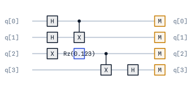
Example circuit plot.

This circuit is deliberately a mixed bag — H, X, CX, a parameterised Rz and a measurement layer — because every option below is easier to judge when there is more than one kind of gate on the page. The rest of this page reuses it.

Note

All OpenQARP Block objects have a plot() method that calls the plotting function on the block’s flat command stream.

Parameters Reference

The plot function accepts the following parameters:

Basic Parameters:

• circ: The circuit or Block to be plotted.

• figsize: The size of the figure in inches (width, height). If None, the size is auto-calculated.

• save_fig: The path to save the figure. If None, the figure is not saved.

• color_scheme: Color scheme for gates. See Color Schemes section.

• spacing: Horizontal spacing between gates. If None, uses default from config.

Layout Parameters:

• flatten_layers: If True, all gates are displayed in optimized horizontal positions. If False, gates are displayed in their original layer structure.

• invert_order: If True, the order of the qubits is inverted (highest index at top). If False, lowest index is at top.

• decompose_boxes: If True, container-style sub-blocks (composites, controlled blocks) are decomposed into their constituent gates before rendering.

Display Parameters:

• scrollable: If True, the plot is displayed in a scrollable HTML container (useful for large circuits in Jupyter).

• use_latex: If True, uses LaTeX for rendering text. Requires LaTeX installation.

• verbose: If True, prints additional information about the plotting process.

Label and Inspection Parameters:

• label_mode: How to handle gate labels. See Label Modes section.

• show_gate_indices: If True, displays small index numbers near each gate for identification.

• return_plotter: If True, returns the CircuitPlotter instance for querying gate information.

• inner_index: Index or path to zoom into box gates. See Inspecting Box Gates section.

Basic Plotting Examples

The examples below reuse the block built in Quick Start above.

Default Plot:

# Simple plot with default settings
plot(block)

Default plot output.

Custom Figure Size:

# Specify figure size (width, height) in inches
plot(block, figsize=(10, 4))

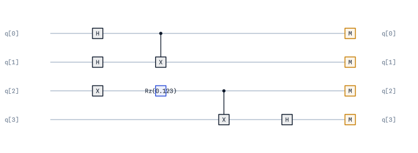
Plot with custom figure size (10, 4).

Adjusting Spacing:

# Default spacing
plot(block, spacing=0.25)

# Tighter spacing
plot(block, spacing=0.15)

# Wider spacing
plot(block, spacing=0.5)

Default spacing (0.25).

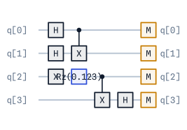
Tight spacing (0.15).

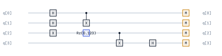
Wide spacing (0.5).

Layout Options

Flatten Layers:

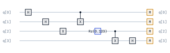
When flatten_layers=True (default), gates are positioned to minimize horizontal space. When False, gates maintain their original layer structure.

# Flattened layout (default) - optimizes horizontal positions
plot(block, flatten_layers=True)

# Consecutive layers - preserves original structure
plot(block, flatten_layers=False)

Flattened layers (flatten_layers=True).

Consecutive layers (flatten_layers=False).

Invert Qubit Order:

Control whether qubit 0 appears at the top or bottom of the plot.

# Default order - qubit 0 at top
plot(block, invert_order=False)

# Inverted order - qubit 0 at bottom
plot(block, invert_order=True)

Default qubit order (invert_order=False).

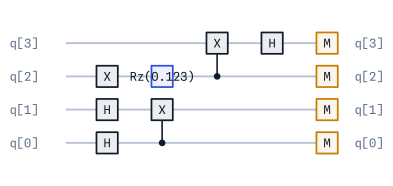
Inverted qubit order (invert_order=True).

Decompose Box Gates:

Container-style sub-blocks (composite blocks, controlled blocks) can be shown as boxes or decomposed into their constituent gates.

This is the one option that needs a circuit with structure to show: block above is a flat list of gates and has no boxes to open, so the example below composes a sub-block first.

from qarp.blocks import CompositeBlock, HypergraphStateBlock, ReadoutBlock

state = HypergraphStateBlock(edges=[(0, 1), (2, 3), (1, 2, 3)], n_qubits=4).build()
boxed_block = CompositeBlock([state, ReadoutBlock(n_qubits=4)], n_qubits=4).build()

# Show box gates as boxes
plot(boxed_block, decompose_boxes=False)

# Decompose box gates into constituent gates
plot(boxed_block, decompose_boxes=True)

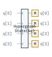
Box gates shown as boxes (decompose_boxes=False).

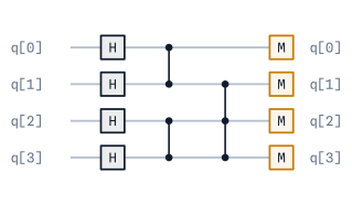
Box gates decomposed (decompose_boxes=True).

Label Modes

The label_mode parameter controls how gate labels are displayed. This is useful for managing label overlaps in complex circuits.

from qarp.plotting import plot
from qarp.plotting import LabelMode

Truncate Mode:

Shows only gate names without parameters. Safest option to avoid overlaps.

# e.g., "Ry(0.123456789*pi + theta)" becomes "Ry"
plot(block, label_mode=LabelMode.TRUNCATE)

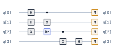
Truncate mode - gate names only.

Smart Mode (Default):

Intelligently positions labels to avoid overlaps, breaking long labels into multiple lines if needed.

plot(block, label_mode=LabelMode.SMART)

Smart mode - intelligent label positioning.

Full Mode:

Displays full labels without any adjustment. May cause overlaps in dense circuits.

plot(block, label_mode=LabelMode.FULL)

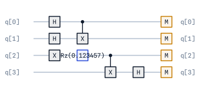
Full mode - complete labels (may overlap).

Gate Indexing and Inspection

The plotting module provides tools to identify and inspect individual gates in a circuit. A multi-gate SimpleBlock embedded in a CompositeBlock renders as one “box” gate rather than being inlined — this section builds a two-level nested example (a box containing more boxes) to demonstrate that:

from qarp.blocks import SimpleBlock, CompositeBlock

# Innermost boxes: two 2-gate leaf blocks.
bell = SimpleBlock(2, name="bell")
bell.h(0)
bell.cx(0, 1)
bell.build()

extra = SimpleBlock(2, name="extra")
extra.z(0)
extra.z(1)
extra.build()

# Middle box: wraps both of the above, so it is itself a multi-gate sub-block.
middle = CompositeBlock([bell, extra], n_qubits=2, name="middle").build()

prep = SimpleBlock(4, name="prep")
prep.h(2)
prep.h(3)
prep.build()

# Outer circuit: two box gates, [prep, middle].
nested_block = CompositeBlock([prep, middle], n_qubits=4, name="outer").build()

Displaying Gate Indices:

Use show_gate_indices=True to display small index numbers near each gate:

plot(nested_block, show_gate_indices=True)

Querying Gate Information:

Use return_plotter=True to get a plotter object that can be used to query gate details:

plotter = plot(nested_block, show_gate_indices=True, return_plotter=True)

# List all gates
plotter.list_gates()
# Output:
# Total gates: 2
# Gate[0]: Block on [q[0], q[1], q[2], q[3]]   (prep)
# Gate[1]: Block on [q[0], q[1]]                (middle)

# Query a specific gate for full information
gate = plotter.query_gate(1)
print(f"Gate type: {gate.gate_type}")      # "Block"
print(f"Full label: {gate.full_label}")    # "Block"
print(f"Qubits: {gate.qubits}")            # ["q[0]", "q[1]"]

Inspecting Box Gates

For container-style sub-blocks (composite blocks, controlled blocks), you can extract and plot their inner circuits using the inner_index parameter. Continuing with nested_block from above:

Single Level Inspection:

# Plot the inner circuit of the box at index 1 (middle)
plot(nested_block, inner_index=1)

Nested Box Inspection:

For circuits with nested box gates, you can provide a path as a list of indices to recursively zoom into nested structures:

# Zoom into nested boxes: box at index 1 (middle) -> box at index 0 inside it (bell)
plot(nested_block, inner_index=[1, 0])

This will:

1. Get the box gate at index 1 from the main circuit (middle)

2. Get the box gate at index 0 from that inner circuit (bell)

3. Plot the final inner circuit — the 2-gate Bell pair (H, CX)

Using Plotter Methods:

For more control, use the plotter’s methods directly:

plotter = plot(nested_block, show_gate_indices=True, return_plotter=True)

# Get the inner circuit (the sub-block / commands at index 1, i.e. `middle`)
inner_circuit = plotter.get_inner_circuit(1)

# Or plot it directly with options
inner_plotter = plotter.plot_inner(1, show_gate_indices=True)
inner_plotter.list_gates()
# Output:
# Total gates: 2
# Gate[0]: Block on [q[0], q[1]]   (bell)
# Gate[1]: Block on [q[0], q[1]]   (extra)

Color Schemes

The color_scheme parameter allows you to customize gate colors. OpenQARP provides several built-in color schemes, including options optimized for different types of color vision deficiency (CVD).

A colour scheme assigns one colour per gate type, so the examples below reuse the mixed-gate block from Quick Start — H, X, CX, Rz and measurements all take a different colour.

Default Scheme:

plot(block, color_scheme='default')

Default color scheme.

Colorblind-Friendly Schemes:

# General colorblind-friendly palette (Wong palette)
# Recommended for publications
plot(block, color_scheme='colorblind')

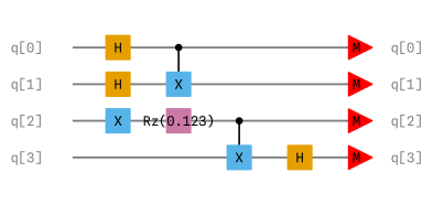
Colorblind-friendly scheme (Wong palette).

# Deuteranopia (green-blind) - most common CVD type
plot(block, color_scheme='deuteranopia')

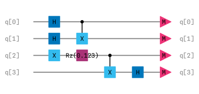
Deuteranopia-friendly scheme.

# Protanopia (red-blind)
plot(block, color_scheme='protanopia')

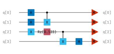
Protanopia-friendly scheme.

# Tritanopia (blue-blind) - rare
plot(block, color_scheme='tritanopia')

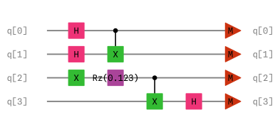
Tritanopia-friendly scheme.

High Contrast and Grayscale:

# High contrast for presentations
plot(block, color_scheme='high_contrast')

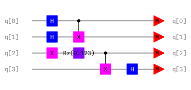
High contrast scheme for presentations.

# Grayscale for black-and-white printing
plot(block, color_scheme='grayscale')

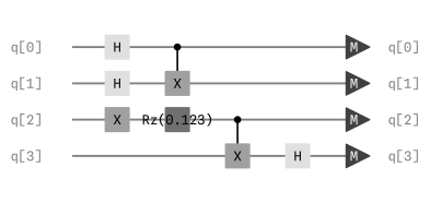
Grayscale scheme for printing.

Custom Color Schemes:

You can provide a custom dictionary mapping gate names (lowercase) to hex colors:

custom_colors = {
    'h': '#FF6B6B',
    'x': '#4ECDC4',
    'cx': '#45B7D1',
    'rz': '#96CEB4',
    'measure': '#FF8579',
    'box': '#EFEFEF',
    # Add other gates as needed
}
plot(block, color_scheme=custom_colors)

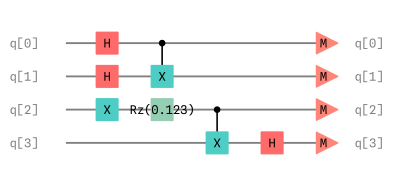
Custom color scheme.

Accessing Color Palettes Directly:

You can import and modify the color dictionaries:

from qarp.plotting.styles import (
    DEFAULT_COLORS,
    COLORBLIND_COLORS,
    PROTANOPIA_COLORS,
    DEUTERANOPIA_COLORS,
    TRITANOPIA_COLORS,
    HIGH_CONTRAST_COLORS,
    GRAYSCALE_COLORS,
    COLOR_SCHEMES,  # Dictionary of all schemes
)

# Customize a scheme
my_colors = COLORBLIND_COLORS.copy()
my_colors['measure'] = '#FF0000'  # Override measure color
plot(block, color_scheme=my_colors)

Display Options

Scrollable Output:

For large circuits in Jupyter notebooks, use the scrollable option:

# Standard output
plot(block, scrollable=False)

# Scrollable HTML container (useful for large circuits)
plot(block, scrollable=True)

LaTeX Rendering:

Enable LaTeX for mathematical text rendering (requires LaTeX installation):

plot(block, use_latex=True)

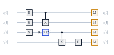
Circuit with LaTeX rendering enabled.

Verbose Output:

Print additional information about the circuit:

plot(block, verbose=True)
# Output:
# Circuit information:
#   Qubits: 4
#   Operations (measurements excluded): 7
#   Global phase: 0.0

Saving Figures

Save plots to files in various formats:

# Save as SVG (recommended for documentation)
plot(block, save_fig="my_circuit.svg")

# Save as PNG
plot(block, save_fig="my_circuit.png")

# Save as PDF
plot(block, save_fig="my_circuit.pdf")

# Combine with other options
plot(block,
     color_scheme='colorblind',
     spacing=0.4,
     save_fig="publication_figure.svg")

Features

OpenQARP’s plotting offers:

• Drastically better performance for large circuits

• Customisable colour schemes including colourblind-friendly options

• Gate indexing and inspection features (non-interactive)

• Several layout control options

• Native rendering of qarpx-IR commands