Graphs

OpenQARP contains some functionality for dealing with graphs, hypergraphs and simplicial complexes, which appear in many places in quantum algorithms and applications. Each native type wraps a standard library object (NetworkX, HyperNetX) and adds the quantum constructions a workflow reaches for — a cost Hamiltonian, a state-preparation block, the sparse matrices behind spectral methods — plus plotting that mimics the plotting of Blocks.

The Graph object

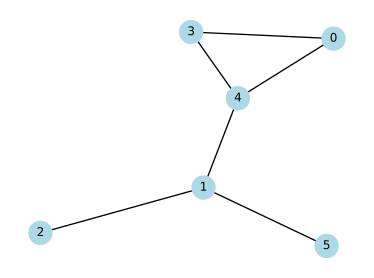
The Graph object is a wrapper for NetworkX Graph objects, that may contain extra functionality which is useful in OpenQARP when building quantum algorithms. For example, OpenQARP graphs have built in plotting function to mimic the plotting of Blocks.

import matplotlib.pyplot as plt
import networkx as nx
from qarp.graphs import Graph as QarpGraph

n_nodes = 6
G = nx.erdos_renyi_graph(n=n_nodes, p=0.5, seed=0)   # seeded for a reproducible figure

qarp_G = QarpGraph(G)

fig, ax = plt.subplots()
nx.draw(qarp_G, ax=ax)

qarp_G.plot(pos=nx.spring_layout(G, seed=0))

Cost Hamiltonian and graph state

Node labels are qubit indices wherever a quantum object is built from a graph, so they must be non-negative integers; they need not be contiguous, and n_qubits is the highest label plus one rather than the node count. to_cost_hamiltonian returns the Ising cost Hamiltonian \(\sum_e w_e Z_i Z_j\) (edge weight from the weight attribute, 1 when absent) — the form QAOA minimises, not the MaxCut objective \(\sum_e w_e (1 - Z_i Z_j)/2\). The two differ by a sign and an offset, so minimising the Hamiltonian maximises the cut, with \(\text{cut} = (\sum_e w_e - \langle H \rangle)/2\). to_graph_state_block returns the graph-state preparation block (a Hadamard on every qubit, then a CZ per edge) and does not need the [hypergraph] extra.

from qarp.algorithms import QAOA
from qarp.graphs import Graph

graph = Graph()
graph.add_edge(0, 1, weight=2.0)
graph.add_edge(1, 2)                          # no weight attribute: counts 1.0

H = graph.to_cost_hamiltonian()               # 2 Z0 Z1 + Z1 Z2
print(graph.n_qubits)                         # 3

qaoa = QAOA(graph, n_layers=2).build()        # QAOA builds the same Hamiltonian
state = graph.to_graph_state_block().build()  # H on every qubit, then CZ per edge

Linear \(Z_i\) terms ride along as the per-node attribute linear, or as an explicit mapping passed as linear=, which replaces the attributes. That is also what makes the operator round trip close: Graph.from_qubit_operator (equal to qubit_operator_to_graph) turns \(Z_i Z_j\) terms into weighted edges and \(Z_i\) terms into linear attributes, so to_cost_hamiltonian recovers the operator up to its constant term, which has no home on a graph. The module-level helper graph_to_cost_hamiltonian accepts a plain networkx.Graph too.

from qarp.graphs import Graph
from qarp.operators import QubitOperator

H = QubitOperator("Z0 Z1", 1.5) + QubitOperator("Z1", 0.3) + QubitOperator("", 2.0)
graph = Graph.from_qubit_operator(H)
print(graph[0][1]["weight"], graph.nodes[1]["linear"])   # 1.5 0.3
print(graph.to_cost_hamiltonian() == H - QubitOperator("", 2.0))   # True

Matrices

The sparse matrices behind spectral partitioning and community detection are methods on the graph: adjacency_matrix, degree_matrix, laplacian_matrix, normalized_laplacian_matrix and the unsigned incidence_matrix, all weighted by the weight attribute, all indexed in node insertion order and all returning a SciPy sparse array (append .toarray() for a dense one). max_modularity_eigenvector returns the leading eigenvector of the modularity matrix; it raises a ValueError on a graph with no edges, where that matrix is undefined, and inherits NetworkX’s convention of ignoring edge weights.

from qarp.graphs import Graph

graph = Graph([(0, 1), (1, 2), (2, 3), (3, 0)])
print(graph.laplacian_matrix().toarray())
print(graph.incidence_matrix().toarray())
print(graph.max_modularity_eigenvector())

The Hypergraph object

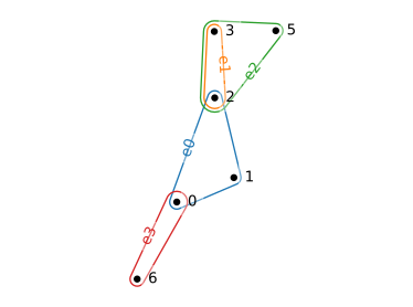
Similarly, the Hypergraph object is a wrapper for HyperNetX Hypergraph objects, also with native plotting functionality. It needs the [hypergraph] extra.

import matplotlib.pyplot as plt
import hypernetx as hnx
from qarp.graphs import Hypergraph as QarpHypergraph

edges = {
    "e0": [0, 1, 2],
    "e1": [2, 3],
    "e2": [2, 3, 5],
    "e3": [0, 6],
}
fig, ax = plt.subplots()

HPG = hnx.Hypergraph(edges)
qarp_HPG = QarpHypergraph(edges)

pos = hnx.drawing.rubber_band.layout_node_link(HPG)
hnx.draw(HPG, pos=pos, ax=ax)
plt.show()

qarp_HPG.plot()

The quantum use of a hypergraph is defining a hypergraph state: a Hadamard on every qubit, then a \(C^{k-1}Z\) per hyperedge of order \(k\). to_state_block returns that HypergraphStateBlock, and n_qubits is the highest vertex index over all edges plus one (vertices are qubit indices, so a sparse labelling still reserves every qubit up to the highest one used). Incidence, dual and adjacency matrices are inherited from HyperNetX; there is no Pauli operator for a hypergraph state, whose stabilisers are non-Pauli for any hyperedge of order three or more.

from qarp.graphs import Hypergraph

HPG = Hypergraph([(0, 1), (1, 2, 3)])
print(HPG.n_qubits)                       # 4
block = HPG.to_state_block().build()      # H^4, then CZ(0, 1) and CCZ(1, 2, 3)

The SimplicialComplex object

We also have SimplicialComplex objects - structures consisting of points, edges, triangles etc., with all their respective faces. This structure is useful for topological data analysis, studying higher-order networks, and defining quantum states with complex correlation patterns beyond pairwise interactions. We can create an initial complex as a list of simplices, add or remove the simplices as needed and plot the complex.

A simplicial complex is closed under faces: every face of a simplex in the complex is itself in the complex. Both the constructor and add_simplex enforce this by adding any missing faces for you, which is why the listing below contains simplices that were never passed in.

from qarp.graphs import SimplicialComplex

simplicial_complex = [
    (0,), (1,), (2,), (3,),  # vertices
    (0, 1), (1, 2), (2, 3),  # edges
    (0, 1, 2),  # triangle
]

qarp_simplicial_complex = SimplicialComplex(simplicial_complex)
print(qarp_simplicial_complex.get_simplices())
qarp_simplicial_complex.plot()

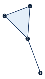
The starting complex: the filled triangle (0, 1, 2) and the pendant edge (2, 3).

Adding a simplex also adds all of its faces:

# Add (0, 1, 3) and all faces, including (0, 1), (0, 3) and (1, 3).
qarp_simplicial_complex.add_simplex((0, 1, 3))
print(qarp_simplicial_complex.get_simplices())
qarp_simplicial_complex.plot()

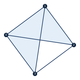
After adding (0, 1, 3), which also brings in (0, 3) and (1, 3): two filled triangles sharing the edge (0, 1).

Removing a simplex also removes every simplex that contains it — that is what keeps the complex closed under faces. Its own faces stay:

# Remove (0, 1).  Both triangles built on it, (0, 1, 2) and (0, 1, 3), go with
# it; the vertices (0,) and (1,) and the other edges stay.
qarp_simplicial_complex.remove_simplex((0, 1))
qarp_simplicial_complex.plot()

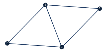
After removing (0, 1). Both triangles that contained it are gone, so nothing is filled any more: what is left is the five remaining edges.

Accessors and cheap topology

The complex is a container (len, iteration in (order, vertices) order, membership that accepts a list in any vertex order) with accessors for its vertices, the neighbours of a vertex, the cofaces of a simplex (every simplex containing it — exactly what remove_simplex deletes), the \(k\)-skeleton and the 1-skeleton as a native Graph. Counts come as num_simplices and the f_vector, and the Euler characteristic \(\chi = \sum_k (-1)^k f_k\) is the cheap topological invariant that tells a filled triangle (\(\chi = 1\)) from a hollow one (\(\chi = 0\)).

from qarp.graphs import SimplicialComplex

sc = SimplicialComplex([(0, 1, 2), (2, 3)])
print(len(sc), (0, 1) in sc, [2, 0] in sc)   # 9 True True
print(sc.vertices(), sc.neighbors(2))          # [0, 1, 2, 3] [0, 1, 3]
print(sc.cofaces((0, 1)))                      # [(0, 1), (0, 1, 2)]
print(sc.skeleton(1).get_simplices())          # vertices and edges only
print(sc.f_vector(), sc.euler_characteristic())   # [4, 4, 1] 1
graph = sc.to_graph()                          # the 1-skeleton, a qarp Graph

The boundary operators \(\partial_k\) and the combinatorial Hodge Laplacians \(L_k = \partial_k^{\mathsf T} \partial_k + \partial_{k+1} \partial_{k+1}^{\mathsf T}\) are available as sparse integer matrices. Rows of \(\partial_k\) index the \((k-1)\)-simplices and columns the \(k\)-simplices, both in get_simplices order, with the sign \((-1)^i\) on the face obtained by deleting the \(i\)-th vertex of the sorted simplex; \(L_0\) is the graph Laplacian of the 1-skeleton. Only the matrices are built — their spectra (Betti numbers, harmonic representatives) are left to the caller.

from qarp.graphs import SimplicialComplex

sc = SimplicialComplex([(0, 1, 2), (2, 3)])
d1 = sc.boundary_matrix(1)                     # 4 vertices x 4 edges, entries in {-1, 0, 1}
d2 = sc.boundary_matrix(2)                     # 4 edges x 1 triangle
print((d1 @ d2).count_nonzero())               # 0: the boundary of a boundary vanishes
print(sc.hodge_laplacian(0).toarray())         # the graph Laplacian of the 1-skeleton
print(sc.hodge_laplacian(1).toarray())