Blocks

Blocks are an abstraction over quantum circuits that implement specific but frequently used functions in larger and more complex circuits. That is, blocks are meant to be readable, reusable, and composable units that you can use to build more complex circuits in a modular way.

We distinguish between two main types of blocks: primitives and state preparation blocks.

• Primitives are designed to be used at any point within the quantum circuit.

• State preparation blocks are intended to be applied at the beginning of the circuit.

Although the API does not enforce this distinction, we strongly recommend adhering to this convention to maintain clarity and consistency in circuit design. That said, if you find a use case where a state preparation block is used somewhere other than the beginning of the circuit, we would love to hear about it!

The SimpleBlock object

The base class for user-defined leaf blocks is SimpleBlock. It extends the nanobind class qx.SimpleBlock and is therefore a qx.Block, so gate-builder methods (self.h(0), self.cx(0, 1), self.rz(0, theta), …) and the C++ command buffer come from the C++ side natively. The Python-side conveniences below are attached from a shared _BlockMixin rather than inherited, so they do not appear in the class’s inheritance chain:

• build() runs build_vanilla(), marks the C++ side built, and finalises sympy bookkeeping.

• flatten() returns the canonical flat command list (list[qx.Command]). Lazy substitutions, replacements, and dagger are applied here.

• dagger() returns a new block (same subclass) representing the adjoint; the reversal is applied lazily at flatten() time.

• to_qasm3(output=None) emits the block as an OpenQASM 3.0 program (optionally writing to a file).

• set_symbols(symbol_parameter_map) returns a new block with the given sympy-symbol values substituted into the commands (lazy; applied at flatten()).

• replace_symbols(new_parameters) returns a new block with each symbol renamed per the dict.

• refresh_symbols(postfix) returns a new block with a postfix added to every symbol name.

• plot() plots the block as a Matplotlib figure.

An example using a single layer of Pauli-Y rotation gates:

from sympy import Symbol
import qarpx as qx
from qarp.blocks import LayerBlock

# define and build the block
thetas = [Symbol(f"theta_{i}") for i in range(5)]
block = LayerBlock(qx.GateType.Ry, 5, parameters=thetas)
block.build()

# non-symbolic ops
block_dagger = block.dagger()
block_qasm = block.to_qasm3()        # OpenQASM 3 string

# symbolic ops
parameter_map = {thetas[j]: j for j in range(len(thetas))}
block_symbolvals = block.set_symbols(parameter_map)

postfix = "a"
block_postfix = block.refresh_symbols(postfix)

new_symbols = [Symbol(f"phi_{i}") for i in range(5)]
symbol_map = {thetas[j]: new_symbols[j] for j in range(len(thetas))}
block_newsymbols = block.replace_symbols(symbol_map)

Controlisation is explicit: wrap any block in ControlledBlock(inner, num_controls, ctrl_state). No other constructor accepts control arguments, so a block’s circuit never depends on the container it is placed in. The wrapped block is num_controls qubits wider than inner: the controls occupy its lowest indices 0 .. num_controls - 1 and the inner block’s qubits follow in their original order, shifted up by num_controls. ctrl_state lists one bool per control in that same order (qubit 0 first, defaulting to all True), and target_qubits on the ControlledBlock places the widened block, controls first — so a one-control wrap of a 4-qubit u with target_qubits=[0, 2, 3, 4, 5] puts the control on qubit 0 and u on 2–5.

Compose with qarp.blocks.CompositeBlock / ControlledBlock / ConditionalBlock. The raw qarpx.CompositeBlock and qarpx.ControlledBlock classes lift a child’s canonical command buffer directly and silently drop a Python block’s pending set_symbols / dagger; they are not a supported composition surface for Python-built blocks and qarp.blocks never re-exports them.

It is possible for the user to inherit from the SimpleBlock class to wrap their own circuits or sub-units of circuits. A few things to keep in mind:

• The constructor of your subclass should accept target_qubits and a keyword-only name (forwarded to SimpleBlock.__init__).

• Define a build_vanilla(self) method that populates self in place by calling the inherited gate builders (self.h(0), self.cx(0, 1), …), it does not return a circuit object.

• For circuits that are composites of sub-blocks you do not need a subclass at all: pass them to CompositeBlock as blocks=[...], as in the next section. Subclassing is only for blocks that compute their own children; those extend CompositeBlockBase and call self.add_child(child_block) from build_vanilla.

The modern interchange surface is to_qasm3() (OpenQASM 3) plus the canonical flat command list returned by flatten().

The CompositeBlock Object

The CompositeBlock allows users to construct a block by combining multiple constituent blocks. Since it inherits from CompositeBlockBase, it is itself a block. The constructor accepts the following arguments:

• blocks: A sequence of blocks in the order they are to be added to the CompositeBlock.

• n_qubits: The total number of qubits the block will need to function correctly.

• target_qubits: Since the CompositeBlock is itself a block, you can define target qubits and reuse your CompositeBlock in another CompositeBlock.

• name: The name of your new block. Defaults to CompositeBlock.

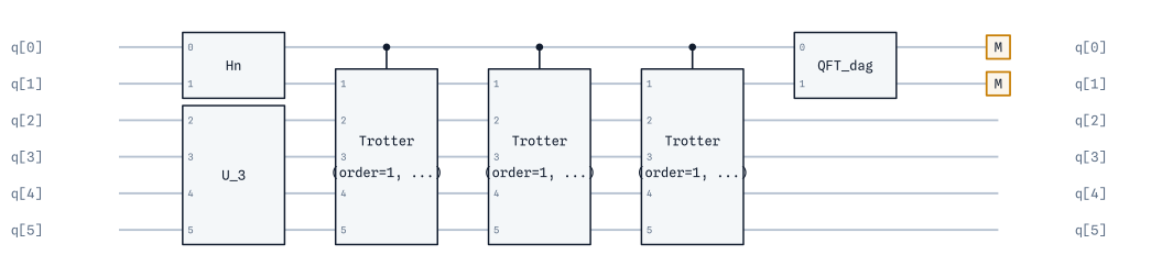
Perhaps the easiest way to understand how the CompositeBlock works is by example. Let’s say we want to construct the textbook QPE circuit, and we have already obtained a qubit operator, which we have stored in the variable qubit_operator. We can build the circuit in just a few lines of code using blocks.

from qarp.blocks import HnBlock, TrotterBlock, ComputationalBasisStateBlock, QFTBlock, ReadoutBlock, CompositeBlock, ControlledBlock
from qarp.operators import QubitOperator
import numpy as np

n_ancilla = 2
n_state = 4
t = 2 * np.pi

# the Hamiltonian whose eigenphases QPE will estimate, any qarp.operators
# QubitOperator on `n_state` qubits works here
qubit_operator = QubitOperator("Z0 Z1", 0.5) + QubitOperator("X2 X3", 0.3)

# construct the blocks.  n_qubits counts the control wire, and the ancilla
# ladder is LSB-first: ancilla 0 takes U^1, ancilla 1 takes U^2.
hn = HnBlock(n_qubits=n_ancilla, target_qubits=[0, 1]).build()
u = TrotterBlock(n_qubits=n_state, operator=qubit_operator, time=t).build()
ctrl_u1 = ControlledBlock(u, 1, [True], target_qubits=[0, 2, 3, 4, 5]).build()
ctrl_u2 = ControlledBlock(u, 1, [True], target_qubits=[1, 2, 3, 4, 5]).build()
iqft = QFTBlock(n_qubits=n_ancilla, target_qubits=[0, 1]).build().dagger()
state = ComputationalBasisStateBlock(basis_state=[1, 1, 0, 0], target_qubits=[2, 3, 4, 5]).build()
measurement = ReadoutBlock(n_qubits=n_ancilla, target_qubits=[0, 1]).build()

# compose them together
qpe_block = CompositeBlock(blocks = [hn, state, ctrl_u1, ctrl_u2, ctrl_u2, iqft, measurement], n_qubits=6).build()

The composed circuit looks like this (see Plotting for how to render a block):

Primitives

qarp.blocks holds the blocks that can be used as part of measurements or algorithms. These blocks are natively backed by qarpx (the compiled qx.Block command buffer described above); interop with other frameworks is available at the edges via to_pytket() / from_pytket() and to_qasm3(). As a block, all primitive blocks inherit n_qubits and target_qubits as optional arguments; control them with ControlledBlock.

AGate Block

AGateBlock implements the A gate, a two-qubit entangling gate. In the qarpx LSB-first basis ordering \(|q_1 q_0\rangle\) (qubit 0 is the least-significant bit, see Endianness) its matrix representation is:

\[\begin{split}A = \begin{pmatrix} 1 & 0 & 0 & 0 \\ 0 & -\cos(\theta) & e^{-i\phi}\sin(\theta) & 0 \\ 0 & e^{i\phi}\sin(\theta) & \cos(\theta) & 0 \\ 0 & 0 & 0 & 1 \end{pmatrix}\end{split}\]

This gate is useful when spanning states after a one-particle excitation, such as in quantum-chemistry applications. For more details, the user is referred to the original paper: Gard et al., npj Quantum Information 6, 10 (2020).

AGateBlock requires arguments theta and phi which define the angles within the A gate.

An example implementation is as follows:

from qarp.blocks import AGateBlock
import numpy as np

a_gate = AGateBlock(theta=0.5 / np.pi, phi=0.3 / np.pi).build()

Brickwork Entangling Block

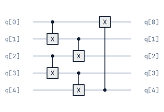
The BrickworkEntanglingBlock entangles qubit \(i\) with qubit \(i+1\) for even values of \(i\), then for odd values of \(i\). It corresponds to the implementation in QURI Parts and to the ‘pairwise’ option in Qiskit, which also does even before odd.

The arguments permit a circular structure (circular=True) in which the last qubit is also entangled with the first ones, and to choose between CZ (use_cz=True) or CX (use_cz=False) for the entanglement. Additionally, the argument n_qubits is required and determines the number of qubits.

An implementation is as follows:

from qarp.blocks import BrickworkEntanglingBlock

n_qubits = 5
block = BrickworkEntanglingBlock(n_qubits=n_qubits, circular=True, use_cz=False).build()

SimpleBlock (ad-hoc circuit construction)

For ad-hoc circuit construction, use SimpleBlock directly: build the gates inline by calling the inherited C++ gate-builder methods.

from qarp.blocks import SimpleBlock

block = SimpleBlock(2, name="HnYn")
block.h(0)
block.h(1)
block.y(0)
block.y(1)
block.build()

Cost Operator Block

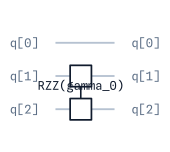
CostOperatorBlock is one of the primitive blocks (besides MixedOperatorBlock) that constitute the QAOA ansatz for finding approximate solutions to combinatorial optimisation problems. Specifically, CostOperatorBlock implements the unitary operator \(U_P(C, \gamma) = e^{-i\gamma C}\), for a given angle \(\gamma\) and Hamiltonian \(C\) corresponding to the cost function of the optimisation problem. Since this block is designed for graph-based problems, problem instances are defined in terms of qarp.graphs.Graph instances.

This block takes as mandatory inputs n_qubits - number of qubits and problem - the graph. Optional inputs are linear_terms - dictionary of single qubit terms in the cost function and symbol_idx - index for symbolic parameter.

An implementation is as follows:

from qarp.blocks import CostOperatorBlock
import networkx as nx

n_nodes = 3
my_graph = nx.erdos_renyi_graph(n=n_nodes, p=0.5)
block = CostOperatorBlock(n_qubits=n_nodes, problem=my_graph).build()

DOS-QPE Block

DOSQPEBlock constructs the purification-based circuit used by Density of States Quantum Phase Estimation (DOS-QPE). Whereas ordinary QPE estimates the phase associated with one prepared eigenstate, DOS-QPE estimates a phase distribution from a mixed probe state. For a maximally mixed probe, the weight of each eigenphase is proportional to its degeneracy.

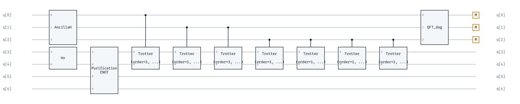
For n_state system qubits and n_ancilla phase qubits, the block uses n_ancilla + 2 * n_state qubits, arranged as follows:

• ancillas 0 through n_ancilla - 1;

• the state register, on which the preparation block and unitary act; and

• a same-size purification register.

The block applies Hadamards to the ancillas, prepares the probe on the state register, and applies one CNOT from each state qubit to its partner in the purification register. It then performs the controlled-unitary phase-estimation ladder and an inverse QFT on the ancillas. The purification qubits are not measured; disregarding them produces the mixed probe state. In particular, preparing HnBlock(n_state) makes this reduced state the maximally mixed state. A different preparation block instead weights the computational-basis components by its squared amplitude magnitudes.

Pass built blocks that both act on n_state qubits: eigenstate prepares the probe and unitary supplies the phase evolution. Set measure=True to append a measurement to each ancilla; sampling and phase-distribution processing are provided by the higher-level DOSQPE algorithm. The controlled unitary must preserve its global phase exactly, because that phase becomes observable under control.

from qarp.operators import JordanWigner
from qarp.operators.models import fermi_hubbard
from qarp.blocks import TrotterBlock, DOSQPEBlock, HnBlock

# Define the number of state and phase-estimation qubits.
n_state = 2
n_ancilla = 3

# Build the unitary evolution for a two-qubit Fermi-Hubbard Hamiltonian.
qham = JordanWigner().encode_operator(fermi_hubbard((1,), t=0.14, U=0.231))
evolution = TrotterBlock(n_qubits=n_state, operator=qham).build()

# Together with the purification CNOTs, this prepares a maximally mixed probe.
probe = HnBlock(n_state).build()

# Create and build the DOS-QPE block
dosqpe_block = DOSQPEBlock(
    eigenstate=probe,
    unitary=evolution,
    n_ancilla=n_ancilla,
    n_state=n_state,
    measure=True,
).build()

The ancilla register resolves phase bins of width \(2^{-n_\mathrm{ancilla}}\).

Givens Block

GivensBlock implements the Givens rotation gate, a two-qubit gate that performs a rotation. In the qarpx LSB-first basis ordering \(|q_1 q_0\rangle\) (qubit 0 is the least-significant bit, see Endianness) its matrix representation is:

\[\begin{split}G = \begin{pmatrix} 1 & 0 & 0 & 0 \\ 0 & \cos(\theta/2) & -\sin(\theta/2) & 0 \\ 0 & \sin(\theta/2) & \cos(\theta/2) & 0 \\ 0 & 0 & 0 & 1 \end{pmatrix}\end{split}\]

It is equivalent to the circuit displayed in Fig. 1.C of Nam et al, npj Quantum Information (2020) 6, 33, for bosonic excitations.

GivensBlock requires input theta, the angle of rotation in radians.

An example implementation is as follows:

from qarp.blocks import GivensBlock
import numpy as np

# Givens rotation gate with rotation angle theta, in radians
givens_gate = GivensBlock(theta=0.5 / np.pi).build()

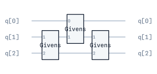
Orbital Rotation Block

OrbitalRotationBlock(u) implements the many-body unitary \(U(u)\) of a real orthogonal single-particle (mode) rotation \(u\),

\[U(u)^\dagger a^\dagger_p U(u) = \sum_q u_{qp}\, a^\dagger_q, \qquad U(u)|0\ldots0\rangle = |0\ldots0\rangle,\]

as an exact — not Trotterized — chain of adjacent-mode GivensBlock gates plus a trailing layer of Z gates absorbing the \(\pm1\) diagonal remainder of the Givens QR decomposition of \(u\). Because every eliminated pair is adjacent, its Jordan-Wigner parity string is empty, so each two-mode rotation is already a plain two-qubit GivensBlock and the construction never needs parity-string uncomputation (Kivlichan et al., Phys. Rev. Lett. 120, 110501 (2018)).

Mode \(p\) is qubit \(p\) under Jordan-Wigner, so the block is JW-only: the same \(u\) under bravyi_kitaev or parity_transform needs different gates. Rows of \(u\) are spin orbitals in interleaved abab order (§1): row \(2\cdot\mathrm{spatial}\) is the \(\alpha\) spin orbital, row \(2\cdot\mathrm{spatial}+1\) its \(\beta\) partner. Expand a spatial-orbital rotation with qarp.operators.integrals.spatial_to_spin_orbital() before use — the same rotation then acts on both spin sublattices.

OrbitalRotationBlock requires the real orthogonal matrix u. Optional dagger emits \(U(u)^\dagger\) (the reversed chain with negated angles — the direction needed to rotate into a measurement basis). The block accepts the standard target_qubits and name options; det(u) = -1 is absorbed by the sign layer rather than rejected.

The following three-mode example rotates into a basis derived from a random orthogonal matrix:

import numpy as np

from qarp.blocks import OrbitalRotationBlock

rng = np.random.default_rng(0)
q, r = np.linalg.qr(rng.normal(size=(3, 3)))
u = q @ np.diag(np.sign(np.diag(r)))  # real orthogonal

orbital_rotation = OrbitalRotationBlock(u).build()
assert orbital_rotation.n_qubits == 3

Haar Random Block

HaarRandomBlock produces Haar-random unitary circuits.

A Haar-random unitary is a unitary matrix drawn uniformly at random from the unitary group \(U(d)\) with respect to the Haar measure, the unique left- and right-invariant probability measure on \(U(d)\). For \(d = 2^n\), this gives a uniformly random \(n\)-qubit unitary. The exact sampling uses the QR decomposition of a random Gaussian matrix (Mezzadri, Notices of the AMS 54, 592 (2007)).

Warning

Implementing a generic Haar-random unitary as a quantum circuit requires \(\mathcal{O}(4^n)\) CNOT gates (Knill, arXiv:quant-ph/9508006; Shende, Bullock & Markov, IEEE Trans. CAD 25, 1000 (2006)). Exact Haar-random synthesis should only be used for small qubit counts. For larger systems, use the approximate t-design construction instead.

A unitary \(t\)-design is an ensemble of unitaries \(\{U_i\}\) that reproduces the first \(t\) moments of the Haar measure (Gross, Audenaert & Eisert, J. Math. Phys. 48, 052104 (2007)). That is, for any polynomial \(f\) of degree at most \(t\) in the entries of \(U\) and \(U^\dagger\):

\[\frac{1}{|S|}\sum_{U_i \in S} f(U_i) = \int_{U(d)} f(U)\, d\mu(U)\]

Local random circuits of depth \(\mathcal{O}(n \cdot t)\) on a 1-D chain form approximate unitary \(t\)-designs (Brandao, Harrow & Horodecki, Commun. Math. Phys. 346, 397 (2016)), making them substantially more efficient on a quantum computer than exact Haar-random synthesis for most practical applications.

It supports two construction strategies:

1. Exact Haar random (default): samples a unitary from the Haar measure and synthesises a circuit implementing it exactly.

2. Approximate t-design (t_design=t): builds a local random circuit of alternating Haar-random single-qubit gates and nearest-neighbour CX layers, approximating a unitary t-design.

The block requires n_qubits. Optional arguments are t_design (if set, uses approximate construction), depth (number of layers for t-design, defaults to n_qubits * t_design), seed for reproducibility, and real (if True, samples from the orthogonal group instead of the unitary group, exact mode only).

Use get_haar_state() to extract the state \(U|0\dots0\rangle\), and reseed() to generate independent random circuits from the same specification.

Example 1: Exact Haar-random unitary

from qarp.blocks import HaarRandomBlock

block = HaarRandomBlock(n_qubits=3, seed=42).build()
state = block.get_haar_state()

Example 2: Approximate t-design

from qarp.blocks import HaarRandomBlock

block = HaarRandomBlock(n_qubits=4, t_design=2, seed=0).build()

Hadamard Test Block

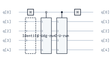
The HadamardTestBlock implements the Hadamard test circuit, which is commonly used to evaluate overlaps, expectation values and transition amplitudes. Which circuit you obtain from the HadamardTestBlock object depends on the input arguments.

The required input arguments are: state - initial state preparation block and unitary - the unitary operator U to test. Optional arguments are: unitary_dagger - unitary to apply for backward evolution, estimate_imaginary - estimate imaginary part if True, real part if False, and measure - whether to add measurement of the ancilla qubit. The standard Block kwarg target_qubits is also accepted.

An example implementation for the real part of an overlap value is shown below:

from qarp.blocks import HadamardTestBlock, IdentityBlock, HnBlock, XnBlock

id = IdentityBlock(n_qubits=4)
u0 = HnBlock(n_qubits=4)
u1 = XnBlock(n_qubits=4)
block = HadamardTestBlock(state=id, unitary=u0, unitary_dagger=u1).build()

Interferometric State and Measurement Blocks

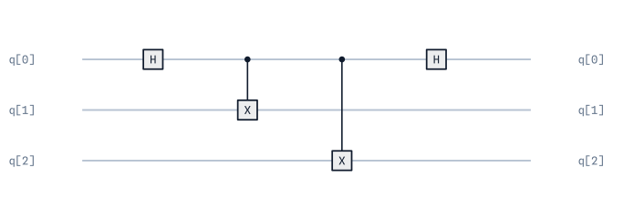
InterferometricStateBlock prepares the measurement-free interferometric transition state

\[\frac{1}{\sqrt{2}}\bigl(|0\rangle|\phi\rangle + |1\rangle|\psi\rangle\bigr),\]

where bra prepares \(|\phi\rangle\) and ket prepares \(|\psi\rangle\) on the same number of qubits. Qubit 0 is the interferometric ancilla and qubits 1..n are the state register. The branch synthesis is delegated to HadamardTestBlock (including its branch-sharing optimization for similar state-preparation circuits), and the optional estimate_imaginary selects which quadrature the ancilla encodes. No basis rotations or measurements are appended, so the block can be embedded in a larger circuit or measured by a caller-specific primitive — for example a custom observable, amplitude estimation, or tomography.

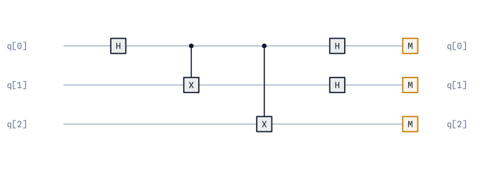
InterferometricMeasurementBlock wraps the same construction with local basis rotations and terminal measurements for a qubit-wise-commuting (QWC) Pauli group. basis maps state-register qubits (indexed from zero, excluding the ancilla) to one of "X", "Y", "Z"; qubits omitted from basis stay in the computational Z basis. Both blocks require bra and ket to act on the same number of qubits and accept the standard name option (neither accepts target_qubits: the ancilla is always the block’s own qubit 0).

from qarp.blocks import IdentityBlock, InterferometricStateBlock, XnBlock

bra = IdentityBlock(n_qubits=2)
ket = XnBlock(n_qubits=2)

block = InterferometricStateBlock(bra=bra, ket=ket).build()

from qarp.blocks import IdentityBlock, InterferometricMeasurementBlock, XnBlock

bra = IdentityBlock(n_qubits=2)
ket = XnBlock(n_qubits=2)

# Measure qubit 0 of the state register in the X basis, qubit 1 in Z.
block = InterferometricMeasurementBlock(
    bra=bra, ket=ket, basis={0: "X", 1: "Z"}
).build()

Hn Block

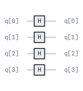
HnBlock implements a superposition state among all the possible quantum basis states, by applying a Hadamard gate in each of the qubits.

It takes n_qubits - number of qubits as an input.

An implementation is as follows:

from qarp.blocks import HnBlock

n_qubits = 4
block = HnBlock(n_qubits=n_qubits).build()

Identity Block

The IdentityBlock object applies an identity to some number of qubits, not impacting their state. This block requires the argument n_qubits - number of qubits. It emits no gates at all — build() produces an empty command list, so the block is a placeholder that reserves a register width (and can be given controls or target qubits like any other) rather than something that draws on the circuit. An example implementation is as follows:

from qarp.blocks import IdentityBlock

identity = IdentityBlock(n_qubits=4).build()
assert len(list(identity.flatten())) == 0

Layer Block

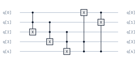
LayerBlock constructs a layer of identical gates across a register of qubits. It supports single-qubit, two-qubit, and three-qubit gates, including both static gates (e.g. H, CX, CCX) and parameterised gates (e.g. Rx, Ry, U).

Required arguments:

• gate_type: A qarpx.GateType specifying which gate to use.

• n_qubits: Total number of qubits in the circuit.

Optional arguments:

• qubit_indices: List of qubit indices where gates are applied (defaults to all qubits).

• overlapping: Number of qubits shared between consecutive multi-qubit gates (default 0). For example, with 2-qubit gates and overlapping=1, gates are applied to qubits (0,1), (1,2), (2,3), ....

• periodic_boundary: If True, wraps around so the last qubit connects back to the first (default False).

• parameters: Parameter values or sympy symbols for parameterised gates. Can be either a single set of parameters (reused for all gates) or a flattened list with parameters for each gate. Angles are in radians.

Example 1: Layer of Hadamard gates

from qarp.blocks import LayerBlock
import qarpx as qx

# Apply H gate to all 4 qubits
h_layer = LayerBlock(gate_type=qx.GateType.H, n_qubits=4).build()

Example 2: Layer of parameterised Ry gates

from qarp.blocks import LayerBlock
from sympy import Symbol
import qarpx as qx

# Create symbolic parameters for each qubit
params = [Symbol(f"theta_{i}") for i in range(4)]
ry_layer = LayerBlock(gate_type=qx.GateType.Ry, n_qubits=4, parameters=params).build()

Example 3: Overlapping 3-qubit gates with periodic boundary

from qarp.blocks import LayerBlock
import qarpx as qx

# CCX gates with 2-qubit overlap and periodic wrapping
block = LayerBlock(gate_type=qx.GateType.CCX, n_qubits=5, overlapping=2, periodic_boundary=True).build()

HEA Block

HEABlock constructs a Hardware-Efficient Ansatz by stacking rotation and entangling layers, as in Kandala et al (Kandala et al., Nature, 549, 242–246 (2017)).

This block takes the following arguments: n_qubits - number of qubits, n_layers - number of HEA layers, real - if True, use only RY rotations, linear - whether to use linear entanglement (True) or brickwork entanglement (False), circular - whether to use periodic boundary conditions for entanglement layers (True) and use_cz - whether to use CZ gates for entanglement (True) or CNOT (False).

An implementation is as follows:

from qarp.blocks import HEABlock

hea = HEABlock(n_qubits=4, n_layers=2, real=True, linear=False, circular=True, use_cz=True).build()

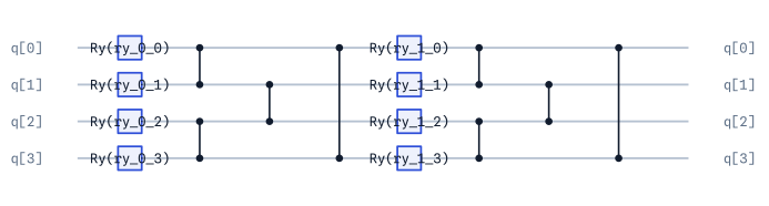
Two layers, each an Ry rotation on every qubit followed by a circular brickwork entangling layer. HEABlock emits these gates directly rather than as one box per layer, so the repeating structure is visible in the figure.

Brickwork PCE Block

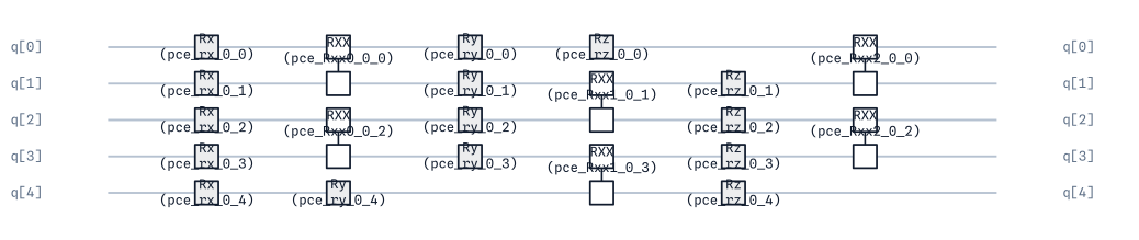
BrickworkPCEBlock constructs the brickwork ansatz used in the original Pauli Correlation Encoding (PCE) paper (Sciorilli et al., Nature Communications 16, 476 (2025)), by stacking n_layers PCE layers. Each layer applies three single-qubit rotation sublayers (Rx, Ry, Rz) interleaved with brickwork \(R_{xx}(\theta) = e^{-i\theta X \otimes X / 2}\) entangling sublayers (native RXX gate). Following BrickworkEntanglingBlock’s tiling, entangling sublayers alternate between even pairs \((0,1),(2,3),\dots\) and odd pairs \((1,2),(3,4),\dots\) — even pairs after Rx, odd pairs after Ry, even pairs again after Rz.

This block takes n_qubits - number of qubits and n_layers - number of PCE layers to stack. It also accepts the standard target_qubits and name options.

An implementation is as follows:

from qarp.blocks import BrickworkPCEBlock

n_qubits = 5
block = BrickworkPCEBlock(n_qubits=n_qubits, n_layers=1).build()

Symmetry Preserving Ansatz Block

SPABlock builds a layered symmetry-preserving ansatz from two-qubit separable-pair gates. These gates leave the zero- and two-excitation basis states unchanged while mixing the one-excitation subspace, making the ansatz useful when the corresponding excitation-number symmetry should be retained.

Choose the gate family with real:

• real=True uses one-parameter RSPBlock gates and keeps the circuit real-valued;

• real=False uses two-parameter AGateBlock gates, adding a phase parameter to the variational freedom.

Each of the n_layers layers applies an entangler to adjacent qubit pairs. With linear=True, the pairs are (0, 1), (1, 2), .... With linear=False, the block uses brickwork ordering: odd pairs first, followed by even pairs. Setting circular=True additionally applies the closing pair (n_qubits - 1, 0) in every layer. For an even number of qubits, a non-circular layer contains n_qubits - 1 pair gates and a circular layer contains n_qubits.

The block carries one symbolic spa_theta_<layer>_<i>_<j> parameter per pair in real mode, and both spa_theta and spa_phi parameters per pair otherwise. It also accepts the standard target_qubits and name options.

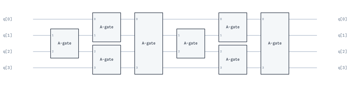
The following example builds a two-layer, circular brickwork ansatz of A-gates:

from qarp.blocks import SPABlock

spa = SPABlock(
    n_qubits=4,
    n_layers=2,
    real=False,
    linear=False,
    circular=True,
).build()

Linear Combination of Unitaries and Block Encoding

LinearCombinationUnitaries decomposes a dense matrix into Pauli strings,

\[A = \sum_i c_i P_i,\]

where each \(P_i\) is a tensor product of I, X, Y, and Z. A matrix whose dimensions are not a power of two is zero-padded to the next square power-of-two dimension by default. The decomposition preserves complex coefficients. Strings are qubit-ordered like QubitOperator terms — character \(k\) acts on qubit \(k\), and A is read in the qarpx LSB basis (row/column bit \(k\) is qubit \(k\)), so 'XI' is \(X_0\) and 'IX' is \(X_1\). The full LCU API is covered in Operators.

BlockEncodingBlock turns that LCU into a unitary circuit. It first prepares the ancilla amplitudes \(\sqrt{|c_i|/\lambda}\), applies the selected Pauli term and its coefficient phase, then unprepares the ancillas. Here \(\lambda = \sum_i |c_i|\), available as lambda_norm (or lambda_factor() for compatibility). Consequently, the all-zero ancilla sector obeys

\[(\langle 0|_\mathrm{anc} \otimes I) U (|0\rangle_\mathrm{anc} \otimes I) = A / \lambda.\]

Pass either a dense numpy.ndarray, a QubitOperator, or explicit keyword-only coefficients and unitaries. The LCU requires max(1, ceil(log2(number_of_terms))) ancilla qubits; the remaining qubits form the target register.

The following example uses a two-qubit, Hamiltonian-like matrix with four Pauli terms. It therefore uses two LCU ancillas and two target qubits, then checks the projected sector:

import numpy as np
import qarpx as qx

from qarp.blocks import BlockEncodingBlock
from qarp.operators import LinearCombinationUnitaries

identity = np.eye(2, dtype=complex)
x = np.array([[0, 1], [1, 0]], dtype=complex)
y = np.array([[0, -1j], [1j, 0]], dtype=complex)
z = np.diag([1, -1]).astype(complex)

# A = 0.35 XX - 0.20 YY + 0.15 ZI + 0.10 IZ.
A = (
    0.35 * np.kron(x, x)
    - 0.20 * np.kron(y, y)
    + 0.15 * np.kron(z, identity)
    + 0.10 * np.kron(identity, z)
)
decomposition = LinearCombinationUnitaries(A).decomposition()
assert {pauli for pauli, _ in decomposition} == {"XX", "YY", "ZI", "IZ"}

block_encoding = BlockEncodingBlock(A, name="Block encoding").build()
assert block_encoding.num_controls == 2
assert block_encoding.n_qubits == 4
full_unitary = np.asarray(
    qx.QarpSimulator().unitary_matrix(
        block_encoding.flatten(), block_encoding.n_qubits
    )
)

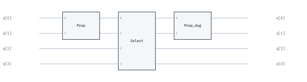
The ancilla register occupies qubits 0 through num_controls - 1 in qarpx’s LSB convention, so the ancilla = 0 sector is strided, not the contiguous top-left corner. No bit reversal is involved: A is read in the same LSB basis the circuit uses (see Endianness). Extract the sector as follows:

n_anc = block_encoding.num_controls
n_target = block_encoding.n_qubits - n_anc
idx = [i * 2**n_anc for i in range(2**n_target)]
recovered = full_unitary[np.ix_(idx, idx)] * block_encoding.lambda_norm

assert np.allclose(recovered, A, atol=1e-12)

Linear Entangling Block

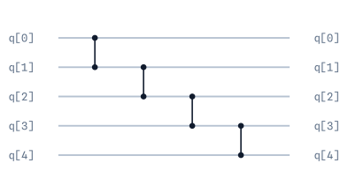
LinearEntanglingBlock entangles qubit \(i\) with the next qubit \(i+1\) for all values of \(i\). Similar to BrickworkEntanglingBlock, LinearEntanglingBlock allows two optional parameters: (circular=True), to entangle the first and last qubit, and (use_cz=True) or (use_cz=False), to use CZ or CX respectively as the entangling gate. The parameter n_qubits is not optional and determines the number of qubits.

An implementation is as follows:

from qarp.blocks import LinearEntanglingBlock

n_qubits = 5
block = LinearEntanglingBlock(n_qubits=n_qubits, circular=False, use_cz=True).build()

Readout Block

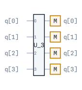
ReadoutBlock is a type of SimpleBlock for appending measurements to a circuit of a given number of qubits n_qubits.

Let’s just create a very simple circuit to demonstrate:

from qarp.blocks import ReadoutBlock, ComputationalBasisStateBlock, CompositeBlock

state = ComputationalBasisStateBlock([1, 1, 0, 0]).build()
meas = ReadoutBlock(n_qubits=4)

block = CompositeBlock([state, meas]).build()

Mixed Operator Block

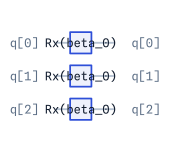
MixedOperatorBlock is part of the QAOA ansatz, and it applies a layer of \(R_x\) rotation gates to \(n\) qubits. Specifically, MixedOperatorBlock implements the unitary operator \(U_M(X, \beta) = \bigotimes_{i=1}^n e^{-i\beta X_i / 2}\), where the rotation angle \(\beta\) is given in radians.

The block parameters are n_qubits, for the number of qubits, and symbol_idx, as an optional parameter specifying the layer index of \(\beta\).

Example:

from qarp.blocks import MixedOperatorBlock

n_nodes = 3
block = MixedOperatorBlock(n_qubits=n_nodes).build()

Paired Unitary Coupled Cluster Doubles (UPCCD) Block

UPCCDBlock implements the paired unitary coupled-cluster doubles (UPCCD) ansatz for closed-shell fermionic systems under an interleaved Jordan–Wigner encoding. For spatial orbital \(p\), qubits 2 * p and 2 * p + 1 represent the alpha and beta spin orbitals, respectively. The block applies Givens rotations between occupied and virtual alpha orbitals, then CNOTs from every alpha qubit to its beta partner to restore the paired occupation.

basis_state defines the closed-shell reference (a plain list of 0s and 1s) that determines the allowed paired excitations. It must have an even number of entries, equal alpha/beta occupations, and an Aufbau ordering; for example, [1, 1, 0, 0, 0, 0] represents one occupied pair in three spatial orbitals. It is not the state-preparation input to the circuit. Instead, prepare the alpha-only reference ([1, 0, 0, 0, 0, 0] in this example) before applying the UPCCD block, because its final CNOT layer copies alpha occupations to beta qubits.

Without t2, one symbolic parameter pd<i>_<j> is created for each allowed occupied-to-virtual pair. Supply t2 with shape (number_of_electron_pairs, number_of_virtual_spatial_orbitals) to initialize those parameters. Entries smaller than threshold are omitted. The block also accepts the standard target_qubits and name options.

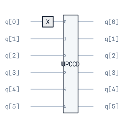
The following six-qubit example has one occupied pair and two virtual orbitals:

import numpy as np

from qarp.blocks import CompositeBlock, ComputationalBasisStateBlock, UPCCDBlock

closed_shell_reference = [1, 1, 0, 0, 0, 0]
alpha_reference = [1, 0, 0, 0, 0, 0]
t2 = np.array([[0.12, -0.07]])

upccd = UPCCDBlock(basis_state=closed_shell_reference, t2=t2).build()
reference = ComputationalBasisStateBlock(alpha_reference)
ansatz = CompositeBlock([reference, upccd], n_qubits=6).build()

# Substitute the supplied paired-double amplitudes in the composite circuit.
ansatz_with_amplitudes = ansatz.set_symbols(upccd.symbol_parameter_map)

Pauli Block

PauliBlock encapsulates a Pauli string (a tensor product of Pauli operators) into a reusable block. This is useful for applying Pauli operators in algorithms, preparing measurement bases, or constructing Hamiltonian terms.

Required arguments:

• pauli_string: The Pauli operators to apply. Can be specified in two formats:

  • String format: A string like "XYZZ" where each character corresponds to a qubit (e.g. qubit 0 gets X, qubit 1 gets Y, etc.). Use "I" for identity.

  • Dictionary format: A dict mapping qubit indices to operators, e.g. {0: "X", 2: "Z"} applies X to qubit 0 and Z to qubit 2 (other qubits unchanged).

Optional arguments:

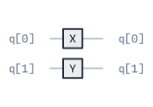
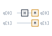
• coefficient: Complex coefficient for the Pauli term. The phase of the coefficient is applied as a global phase.

• phase: Global phase in radians (mutually exclusive with coefficient).

• n_qubits: Total number of qubits (required for dictionary format if indices don’t cover all qubits).

• change_basis: If True, emits basis-change gates for measurement (H for X-basis, Sdg then H for Y-basis, nothing for Z) instead of the Pauli operators themselves, so PauliBlock("XZ", change_basis=True) yields a single H rather than X, Z.

• measure: If True, appends measurements to all qubits.

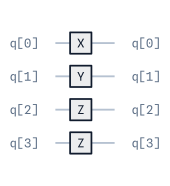
Example 1: Simple Pauli string

from qarp.blocks import PauliBlock

# Apply X⊗Y⊗Z⊗Z to 4 qubits
pauli_block = PauliBlock("XYZZ").build()

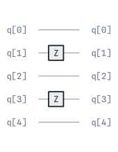
Example 2: Sparse Pauli string using dictionary format

from qarp.blocks import PauliBlock

# Apply Z to qubits 1 and 3 only (in a 5-qubit system)
pauli_block = PauliBlock({1: "Z", 3: "Z"}, n_qubits=5).build()

Example 3: Pauli term with coefficient (for Hamiltonian simulation)

from qarp.blocks import PauliBlock

# Pauli term with complex coefficient 0.5j
pauli_block = PauliBlock("XY", coefficient=0.5j).build()

Example 4: Measurement in the Pauli basis

from qarp.blocks import PauliBlock

# Prepare measurement in the X⊗Z basis
measurement_block = PauliBlock("XZ", change_basis=True, measure=True).build()

Phase Shift Block

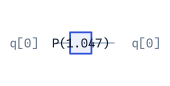
PhaseShiftBlock implements the single-qubit phase gate

\[\begin{split}P(\theta) = \begin{pmatrix}1 & 0 \\ 0 & e^{i\theta}\end{pmatrix}.\end{split}\]

It leaves \(|0\rangle\) unchanged and multiplies \(|1\rangle\) by \(e^{i\theta}\). It is therefore a relative phase, not a global phase. The required phase angle is in radians. Use target_qubits to place the one-qubit block within a larger circuit; wrap it in ControlledBlock for a controlled version.

For example:

import numpy as np
import qarpx as qx

from qarp.blocks import PhaseShiftBlock

phase = np.pi / 3
block = PhaseShiftBlock(phase=phase).build()

unitary = np.asarray(qx.QarpSimulator().unitary_matrix(block.flatten(), block.n_qubits))
expected = np.diag([1.0, np.exp(1j * phase)])
assert np.allclose(unitary, expected)

Projected Control Phase Block

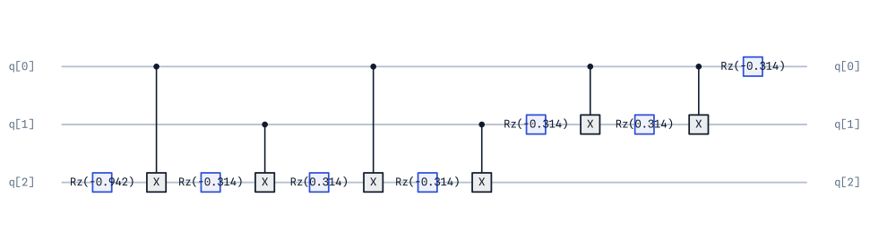
ProjectedControlPhaseBlock implements a diagonal, subspace-selective phase operation. For a dim-dimensional prefix of the computational basis, it realizes

\[D(\phi, d) = \operatorname{diag}(\underbrace{e^{i\phi}, \ldots, e^{i\phi}}_{d}, \underbrace{e^{-i\phi}, \ldots, e^{-i\phi}}_{2^n-d}).\]

Here phase is \(\phi\) in radians, dim is \(d\), and n_qubits is \(n\). The prefix contains computational-basis indices 0 through dim - 1; these indices follow qarpx’s LSB qubit convention. dim may range from 0 to 2**n_qubits. At either endpoint the operation is only a global phase; otherwise the two subspaces acquire a relative phase \(e^{2 i \phi}\).

The block uses diagonal-unitary synthesis, so numerical comparisons should disregard an overall global phase. It also accepts the standard target_qubits and name options. For two qubits with dim=1, the ideal diagonal is

\[\begin{split}R = \begin{pmatrix} e^{i \phi} & 0 & 0 & 0 \\ 0 & e^{-i\phi} & 0 & 0 \\ 0 & 0 & e^{-i\phi} & 0 \\ 0 & 0 & 0 & e^{-i\phi} \end{pmatrix}\end{split}\]

The following three-qubit example phases the first three basis states:

import numpy as np
import qarpx as qx

from qarp.blocks import ProjectedControlPhaseBlock

phase = np.pi / 5
dim = 3
n_qubits = 3
block = ProjectedControlPhaseBlock(phase=phase, dim=dim, n_qubits=n_qubits).build()

unitary = np.asarray(qx.QarpSimulator().unitary_matrix(block.flatten(), n_qubits))
expected = np.array(
    [np.exp(1j * phase)] * dim
    + [np.exp(-1j * phase)] * (2**n_qubits - dim)
)

# The synthesized circuit can differ only by an overall global phase.
assert np.allclose(unitary, np.diag(np.diag(unitary)))
assert np.allclose(np.diag(unitary) / unitary[0, 0], expected / expected[0])

Projector Blocks

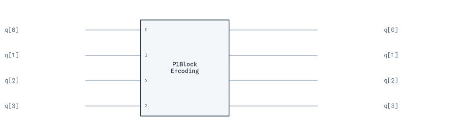
OpenQARP provides at the moment four symmetry-projector blocks:

• ParticleNumberProjectorBlock(n_qubits, Npart) selects the sector with exactly Npart occupied spin orbitals, where Npart is an integer from zero through n_qubits.

• SzProjectorBlock(n_qubits, Ms) selects an eigenvalue Ms of total \(S_z\). Spin orbitals use the alternating convention in which even qubits are alpha orbitals and odd qubits are beta orbitals.

• SyProjectorBlock(n_qubits, My) selects an eigenvalue My of total \(S_y\). It uses adjacent alpha/beta pairs and therefore requires an even number of system qubits.

• SpinSquaredProjectorBlock(n_qubits, S, Ms=...) selects both the \(S^2=S(S+1)\) and \(S_z=M_s\) sectors. It requires an even number of system qubits and valid integer or half-integer spin quantum numbers.

These blocks implement the LCU symmetry-projector constructions described by Khinevich and Mizukami in Symmetry-Adapted State Preparation for Quantum Chemistry on Fault-Tolerant Quantum Computers, using equivalent OpenQARP phase conventions. OpenQARP extends that construction with a standalone \(S_y\) projector and explicit support for half-integer-spin sectors. The classes documented here use the LCU route with internal implementations; not the alternative GQSP or GQSVT projector constructions.

These are unitary block encodings of non-unitary projectors. If \(P\) denotes the desired projector and \(U_P\) the complete circuit, then

\[\langle 0\ldots0|_{\mathrm{anc}} U_P |0\ldots0\rangle_{\mathrm{anc}} = \frac{P}{\lambda}.\]

The LCU ancillas are the lowest-index qubits and the system register is exposed as system_qubits. num_controls gives the number of LCU ancillas and lambda_norm (also returned by lambda_factor()) is \(\lambda\). Consequently, applying the full unitary does not deterministically project a state: the projector is obtained from the all-zero ancilla branch, with success probability \(\|P|\psi\rangle\|^2/\lambda^2\).

The particle-number, \(S_z\), and \(S_y\) blocks use exact roots-of-unity filters with n_qubits + 1 LCU terms. The spin-squared block uses an Euler-angle quadrature with n_alpha * n_beta * n_gamma terms; its positive grid sizes may be overridden when a different accuracy/resource trade-off is required. All projector blocks expose n_terms, lcu_coefficients, and unitaries for inspecting the decomposition.

The following two-system-qubit example extracts the one-particle projector from the all-zero ancilla block and checks it against its exact matrix:

import numpy as np
import qarpx as qx

from qarp.blocks import ParticleNumberProjectorBlock

projector = ParticleNumberProjectorBlock(
    n_qubits=2, Npart=1, name="P1"
).build()
unitary = np.asarray(
    qx.QarpSimulator().unitary_matrix(projector.flatten(), projector.n_qubits)
)

# qarpx is LSB-first, so fixing the low ancilla bits to zero gives
# strided system-register indices.
zero_ancilla = [
    system_state * 2**projector.num_controls
    for system_state in range(2**projector.n_system_qubits)
]
encoded = unitary[np.ix_(zero_ancilla, zero_ancilla)]
recovered_projector = projector.lambda_norm * encoded

expected = np.diag([0.0, 1.0, 1.0, 0.0])
assert np.allclose(recovered_projector, expected, atol=1e-10)

QAOABlock

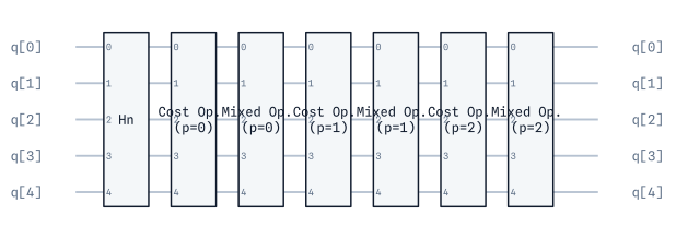
QAOABlock is a type of CompositeBlock that constructs an ansatz for the Quantum Approximate Optimization Algorithm (QAOA) with \(p\) layers. It consists of an HnBlock block across all qubits to initially create a superposition between all computational basis states, followed by \(p\) layers of CostOperatorBlock and MixedOperatorBlock blocks. The resulting circuit contains a total of \(2p\) parameters, which are optimized during the algorithm’s execution.

Required parameters of QAOABlock are as follows: n_qubits, the number of qubits; n_layers, the number of QAOA layers \(p\); and, problem, a graph defining the optimisation problem instance. Optional parameters are as follows: linear_terms, a dictionary of linear (single-qubit) terms in the cost function; and, use_rzz, to emit each cost term as a native RZZ rotation (use_rzz=True) or as its CX·Rz·CX decomposition (use_rzz=False).

The example below shows how to create a QAOABlock from a graph, where the number of qubits corresponds to the number of nodes in the graph.

First, we create a random graph using NetworkX:

import networkx as nx

n_nodes = 5
n_edges = 20
seed = 1234

G = nx.gnm_random_graph(n_nodes, n_edges, seed=seed)
for u, v in G.edges:
    G[u][v]['weight'] = 2

Next, we construct the QAOABlock based on the graph and visualize it using OpenQARP’s built-in plotting functionality:

from qarp.blocks import QAOABlock

block = QAOABlock(n_qubits=n_nodes, n_layers=3, problem=G, use_rzz=True).build()
block.plot()

QFT Block

QFTBlock implements the quantum fourier transform (QFT):

\[|j\rangle \longrightarrow \frac{1}{\sqrt{N}} \sum_{k=0}^{N-1} e^{2\pi i j k / N} |k\rangle\]

The inverse quantum fourier transform can be found by taking the dagger of the QFT.

For inputs the block takes n_qubits - number of qubits.

An example implementation is as follows:

from qarp.blocks import QFTBlock

n_qubits = 4
qft = QFTBlock(n_qubits).build()

QPE Block

QPEBlock builds the circuit underlying quantum phase estimation. Given an eigenstate \(|\psi\rangle\) of a unitary \(U\),

\[U|\psi\rangle = e^{2\pi i\phi}|\psi\rangle,\]

it writes an \(n_\mathrm{ancilla}\)-bit estimate of \(\phi\) into an ancilla register. The block itself builds a circuit; sampling and selecting the most probable phase are handled by the higher-level QPE algorithm.

For n_state system qubits and n_ancilla phase qubits, the layout is n_ancilla + n_state qubits:

• ancillas 0 through n_ancilla - 1;

• a state register containing the remaining qubits.

The block applies Hadamards to the ancillas, prepares eigenstate on the state register, applies controlled \(U^{2^i}\) for each ancilla \(i\), and finishes with an inverse QFT. Set measure=True to append measurements to the ancillas only. The phase-bin spacing is \(2^{-n_\mathrm{ancilla}}\); phases not on that grid are returned as a distribution over nearby bins.

Both eigenstate and unitary must act on n_state qubits. The unitary must also preserve its global phase exactly: a global phase becomes observable when the unitary is controlled.

The following example uses an exactly representable phase, \(\phi=3/8\):

import numpy as np

from qarp.blocks import ComputationalBasisStateBlock, PhaseShiftBlock, QPEBlock

phase = 3 / 8
n_state = 1
n_ancilla = 3

# P(2πφ)|1> = exp(2πiφ)|1>.
eigenstate = ComputationalBasisStateBlock([1]).build()
unitary = PhaseShiftBlock(phase=2 * np.pi * phase).build()

qpe_block = QPEBlock(
    eigenstate=eigenstate,
    unitary=unitary,
    n_ancilla=n_ancilla,
    n_state=n_state,
    measure=True,
).build()

Modular Multiplication Block

ModularMultiplicationBlock(m, N) implements reversible multiplication modulo a small integer as an exact basis permutation on \(n=\lceil\log_2 N\rceil\) LSB-indexed work qubits:

\[\begin{split}|x\rangle \longrightarrow \begin{cases} |m x \bmod N\rangle, & x < N,\\ |x\rangle, & x \geq N. \end{cases}\end{split}\]

Fixing the labels \(x \geq N\) is part of the contract, since a block must define a unitary on the whole register. The multiplier must be coprime to the modulus so that the map is a bijection. The block is phase-exact and therefore safe under ControlledBlock.

from qarp.blocks import ModularMultiplicationBlock

multiply_by_two_mod_five = ModularMultiplicationBlock(2, 5).build()

Warning

The synthesizer enumerates computational-basis labels and lowers each adjacent swap to a wide multi-controlled gate, so its gate count is exponential in the work width. MAX_REFERENCE_WORK_QUBITS caps the width at six (\(N \le 64\)); larger moduli raise ValueError.

Order Finding Block

OrderFindingBlock(a, N) is the measurement-free circuit behind Shor’s algorithm. Its LSB register layout is counting (qubits 0 .. t-1) followed by work (qubits t .. t+n-1), with t = 2n by default. It applies Hadamards to the counting register, prepares the work register in \(|1\rangle\), applies one controlled ModularMultiplicationBlock with multiplier \(a^{2^j} \bmod N\) per counting qubit \(j\), and finishes with the inverse QFTBlock on the counting register. Measuring the counting register samples phases \(s/r\) where \(r\) is the multiplicative order of \(a\) modulo \(N\). No measurement is embedded; a Sampler with measured_qubits=block.counting_qubits marginalises the work register.

import qarp
from qarp.algorithms import Sampler
from qarp.blocks import OrderFindingBlock
from qarp.engines import QarpEngine

block = OrderFindingBlock(2, 15).build()
sampler = Sampler(ket=block, n_shots=qarp.EXACT, measured_qubits=block.counting_qubits)
engine = QarpEngine()
engine.build([sampler])
distribution = engine.run()[0]

The block inherits the six-work-qubit reference limit of ModularMultiplicationBlock. See the Shor section of the algorithms page for the full factoring workflow.

Quantum Signal Processing Block

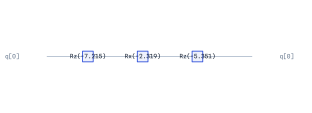
QSPBlock implements a one-qubit quantum-signal-processing sequence for a real signal value \(a\in[-1,1]\). Its signal rotation is \(W(a)=\exp(i\arccos(a)X)\) and the supplied phases insert Z rotations between successive signal rotations. For phases synthesized for a feasible polynomial \(P\), the real part of the upper-left matrix element of the resulting unitary approximates \(P(a)\). See Wang et al. for the phase conventions used here.

QSPBlock is useful for inspecting or composing a QSP sequence after its phase angles have been obtained. P_angles are in radians. QSPAngleFinder numerically finds phases for a polynomial specified by its coefficients in ascending order; as in standard QSP, the requested polynomial must satisfy the relevant parity and boundedness conditions.

The following example synthesizes \(P(x)=x\) and verifies the encoded matrix element:

import numpy as np
import qarpx as qx
from qarp.blocks import QSPBlock, QSPAngleFinder

a = 0.4
phases = QSPAngleFinder([0, 1]).QSP()  # P(x) = x
qsp = QSPBlock(a=a, P_angles=phases).build()

unitary = np.asarray(qx.QarpSimulator().unitary_matrix(qsp.flatten(), qsp.n_qubits))
assert np.isclose(unitary[0, 0].real, a, atol=1e-8)

Qubitization Block

QubitizationBlock constructs the qubitization walk from the LCU block encoding of an operator \(A\) and a reflection on that block encoding’s ancilla register. In OpenQARP, the reflection is applied first in circuit time, so the resulting unitary is

\[W = \operatorname{BE}(A) R_0, \qquad R_0=2|0\ldots0\rangle\langle0\ldots0|-I.\]

A may be an np.ndarray or a QubitOperator. The underlying BlockEncodingBlock encodes \(A/\lambda\), and its normalization is exposed as lambda_factor. For Hermitian \(A\) with eigenvalue \(E\), the walk has eigenphases \(\exp(\mathord{\pm}i\arccos(E/\lambda))\). Therefore, if phase estimation reports a phase \(\theta\) in \([0,1)\), then \(E=\lambda\cos(2\pi\theta)\). The two signs give conjugate phases and the same energy, so the corresponding phase distribution is symmetric about 0 and 0.5.

For example, a two-term one-qubit Hamiltonian needs one LCU ancilla qubit:

from qarp.blocks import QubitizationBlock
from qarp.operators import QubitOperator

hamiltonian = 0.7 * QubitOperator("X0") - 0.3 * QubitOperator("Z0")
walk = QubitizationBlock(hamiltonian, operator_name="H").build()

assert walk.BE.num_controls == 1
assert walk.lambda_factor == 1.0

QSVTBlock

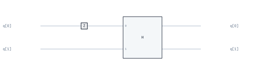
QSVTBlock implements quantum singular value transformation by alternating a block encoding of \(A\) (and its adjoint) with phases conditioned on the LCU ancilla being \(|0\ldots0\rangle\). The phase layers apply \(e^{+i\phi}\) on that subspace and \(e^{-i\phi}\) elsewhere. A phase list of length \(d+1\) specifies a degree-\(d\) transformation.

The current implementation accepts an np.ndarray or a QubitOperator. Array inputs must be square and Hermitian, and the generated block encoding must be real. OpenQARP automatically rescales the input by the block-encoding normalization \(\lambda\); consequently, phase angles transform \(A/\lambda\), not an unnormalised input \(A\). P_angles are in radians and can be obtained with QSPAngleFinder(...).QSVT() for a feasible polynomial.

This example applies \(P(x)=x^2-1\) to a real symmetric two-by-two matrix. It normalizes the matrix explicitly to make the expected projected block unambiguous:

import numpy as np
import qarpx as qx
from qarp.blocks import BlockEncodingBlock, QSVTBlock, QSPAngleFinder

A = np.array([[0.5, 0.3], [0.3, -0.5]])
A /= BlockEncodingBlock(A).lambda_factor()
phases = QSPAngleFinder([-1, 0, 1]).QSVT()
qsvt = QSVTBlock(A, phases).build()

# Extract the block on the |0…0>_ancilla subspace. The ancillas are the low
# qubits (qarpx LSB), so its indices are strided (0, N_anc, 2·N_anc, …), not
# the literal top-left corner; A itself is read in the same LSB basis.
unitary = np.asarray(qx.QarpSimulator().unitary_matrix(qsvt.flatten(), qsvt.n_qubits))
n_ancilla = qsvt.n_qubits - 1
zero_ancilla = [i * 2**n_ancilla for i in range(2)]
transformed_A = unitary[np.ix_(zero_ancilla, zero_ancilla)].real
assert np.allclose(transformed_A, A @ A - np.eye(2), atol=1e-8)

The same strided extraction works for a target register wider than one qubit; see the Block Encoding example above.

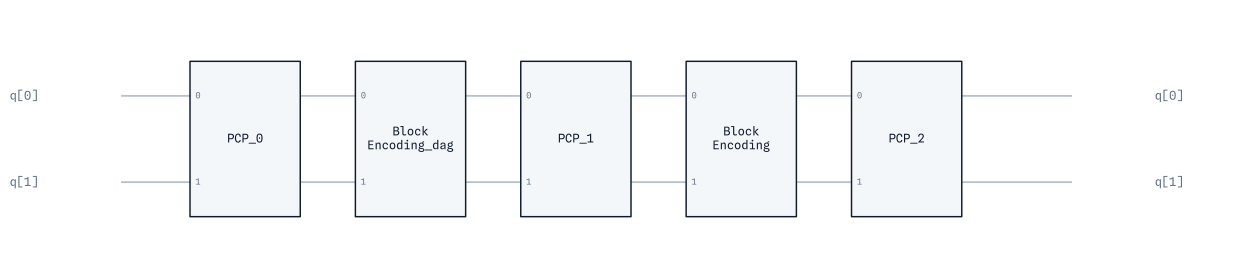
Reflection Block

ReflectionBlock(n_qubits) implements the exact Grover-style reflection

\[R_0=2|0\ldots0\rangle\langle0\ldots0|-I.\]

It gives \(+1\) to \(|0\ldots0\rangle\) and \(-1\) to every other computational-basis state. n_qubits must be at least one. The multi-qubit implementation includes the global sign needed for this exact definition, which matters when the reflection is controlled or composed in a qubitization walk.

The following verifies the diagonal action for three qubits:

import numpy as np
import qarpx as qx
from qarp.blocks import ReflectionBlock

block = ReflectionBlock(n_qubits=3).build()
unitary = np.asarray(qx.QarpSimulator().unitary_matrix(block.flatten(), block.n_qubits))
assert np.allclose(unitary, np.diag([1] + [-1] * 7))

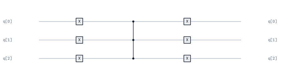
Amplitude Amplification Block

AmplitudeAmplificationBlock implements the phase-exact amplitude-amplification iterate

\[Q = A R_0 A^\dagger O_\mathrm{good},\]

built from a state-preparation unitary A and a good-state phase oracle oracle implementing exactly \(O_\mathrm{good} = I - 2\Pi_\mathrm{good}\), with \(R_0\) supplied by ReflectionBlock. This convention is Eq. (1) of Brassard, Høyer, Mosca and Tapp, Quantum Amplitude Amplification and Estimation, arXiv:quant-ph/0005055. A raw ReflectionBlock about the good subspace implements the exact negative of a good-state oracle; compose it with a gphase(pi) block to restore the sign before using it here.

state_preparation and oracle must act on the same number of qubits, and state_preparation must be deterministic (ancilla_postselection is None), since \(R_0\) reflects about \(|0\ldots0\rangle\) on the whole register. Both inputs are deep-copied at construction, so building this block never mutates either. The keyword-only power (default 1) repeats the iterate as \(Q^\mathrm{power}\); power=0 is the identity. The oracle’s phase convention is the caller’s promise — the constructor checks type and register width but cannot verify the phase semantics without an exponential-size matrix.

from qarp.blocks import AmplitudeAmplificationBlock, HnBlock, SimpleBlock

def phase_oracle(n_qubits, marked_labels):
    # I - 2 Pi_good: flips the sign of each marked computational basis label.
    block = SimpleBlock(n_qubits, name="O_good")
    qubits = list(range(n_qubits))
    for label in marked_labels:
        zero_qubits = [q for q in qubits if not (label >> q) & 1]
        block.x(zero_qubits)
        block.mcz(qubits)
        block.x(zero_qubits)
    return block

state_preparation = HnBlock(n_qubits=2).build()
oracle = phase_oracle(2, [3]).build()  # marks |11>
iterate = AmplitudeAmplificationBlock(state_preparation, oracle).build()

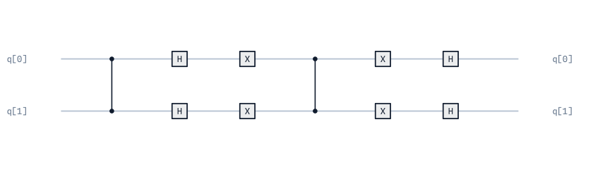
Amplitude Estimation Block

AmplitudeEstimationBlock builds the canonical (measurement-free) quantum amplitude estimation circuit. For A|0...0> = sqrt(1-a)|psi_bad> + sqrt(a)|psi_good> and a phase-exact oracle as above, the embedded AmplitudeAmplificationBlock iterate has eigenphases \(\pm2\theta\) with \(\sin^2\theta = a\); this block applies QPEBlock to that iterate without appending measurements, following Brassard, Høyer, Mosca and Tapp (arXiv:quant-ph/0005055).

For a positive number of estimation qubits n_ancilla, the layout is n_ancilla + n_state qubits: the estimation register occupies qubits 0 .. n_ancilla - 1 and the state register follows it. state_preparation and oracle are subject to the same contract as AmplitudeAmplificationBlock (equal width, deterministic preparation, an exact phase oracle) and are likewise deep-copied and never built, retargeted, or otherwise mutated by the constructor.

from qarp.blocks import AmplitudeEstimationBlock, HnBlock, SimpleBlock

def phase_oracle(n_qubits, marked_labels):
    block = SimpleBlock(n_qubits, name="O_good")
    qubits = list(range(n_qubits))
    for label in marked_labels:
        zero_qubits = [q for q in qubits if not (label >> q) & 1]
        block.x(zero_qubits)
        block.mcz(qubits)
        block.x(zero_qubits)
    return block

state_preparation = HnBlock(n_qubits=2).build()
oracle = phase_oracle(2, [3]).build()
qae = AmplitudeEstimationBlock(state_preparation, oracle, n_ancilla=2).build()
assert qae.n_qubits == 4

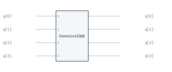
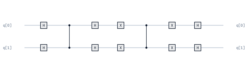
Grover Block

GroverBlock builds uniform-state Grover search for a known number of marked states. It prepares HnBlock across the oracle’s register, then applies the integer number of AmplitudeAmplificationBlock iterates that maximizes \(\sin^2\bigl((2k+1)\theta\bigr)\) around the first optimum, where \(\theta=\arcsin\sqrt{t/N}\), \(N=2^{n_\mathrm{qubits}}\) and \(t\) is n_marked — the uniform-search construction of Grover (arXiv:quant-ph/9605043) with the known-multiple-solution iteration count of Boyer, Brassard, Høyer and Tapp (arXiv:quant-ph/9605034).

oracle must implement exactly \(I - 2\Pi_\mathrm{good}\) (the same contract as AmplitudeAmplificationBlock’s oracle) and is deep-copied at construction; it is not inferred from n_marked. After building, the block exposes n_iterations (the chosen iterate count) and predicted_success_probability.

from qarp.blocks import GroverBlock, SimpleBlock

def phase_oracle(n_qubits, marked_labels):
    block = SimpleBlock(n_qubits, name="O_good")
    qubits = list(range(n_qubits))
    for label in marked_labels:
        zero_qubits = [q for q in qubits if not (label >> q) & 1]
        block.x(zero_qubits)
        block.mcz(qubits)
        block.x(zero_qubits)
    return block

oracle = phase_oracle(2, [3]).build()  # searches for |11>
grover = GroverBlock(oracle, n_marked=1).build()
assert grover.n_iterations == 1

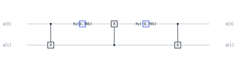
RSP Block

RSPBlock implements the real-valued, symmetry-preserving two-qubit gate used by the real symmetry-preserving ansatz. It preserves excitation number: it leaves \(|00\rangle\) and \(|11\rangle\) unchanged and acts on the single-excitation subspace. In OpenQARP’s LSB qubit convention, its matrix is

\[\begin{split}\operatorname{RSP}(\theta)= \begin{pmatrix} 1 & 0 & 0 & 0 \\ 0 & -\sin\theta & \cos\theta & 0 \\ 0 & \cos\theta & \sin\theta & 0 \\ 0 & 0 & 0 & 1 \end{pmatrix}\end{split}\]

This is the LSB-basis representation of the circuit in Fig. 1 of Ibe et al., Physical Review Research 4, 013173 (2022). At \(\theta=0\), it is the two-qubit SWAP gate. theta is in radians and may be a number, a SymPy symbol, or a linear expression in one symbol.

For example:

import numpy as np
import qarpx as qx
from qarp.blocks import RSPBlock

theta = np.pi / 4
s, c = np.sin(theta), np.cos(theta)
rsp_gate = RSPBlock(theta=theta).build()
unitary = np.asarray(qx.QarpSimulator().unitary_matrix(rsp_gate.flatten(), rsp_gate.n_qubits))
expected = np.array([[1., 0., 0., 0.],
                     [0., -s, c, 0.],
                     [0., c, s, 0.],
                     [0., 0., 0., 1.]])

assert np.allclose(unitary.real, expected, atol=1e-8)

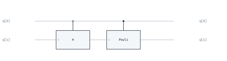
Select Block

SelectBlock applies one unitary to a target register conditional on a selector register. The selector qubits occupy local indices [0, ..., num_controls - 1] and the target qubits follow them. Entries in unitaries are assigned positionally to selector states in lexicographic order of the tuple (q0, q1, ...): with two qubits, the order is 00, 01, 10, 11. This ordering is distinct from ascending integer order because OpenQARP uses q0 as the least-significant qubit.

An entry may be a unitary Block, (phase, Block), or the convenient (phase, pauli_string_or_dict) form. phase is in radians and realizes \(e^{i\,\mathrm{phase}}U\); it is preserved even when SELECT is later controlled. All full-width blocks and Pauli strings must have the same target width. Fewer than \(2^{\mathtt{num\_controls}}\) entries are allowed: unlisted selector states apply the identity.

This one-control example applies H for selector \(|0\rangle\) and \(e^{i\pi/5}Z\) for selector \(|1\rangle\):

import numpy as np
from qarp.blocks import SelectBlock, SimpleBlock

hadamard = SimpleBlock(1, name="H")
hadamard.h(0)
hadamard.build()

select_block = SelectBlock(
    unitaries=[hadamard, (np.pi / 5, "Z")], num_controls=1
).build()
assert select_block.n_qubits == 2  # q0 is selector; q1 is target

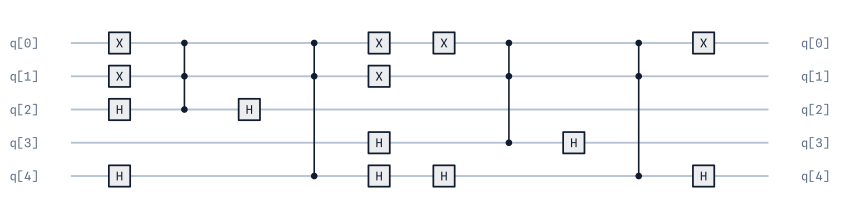
QROM Block

QROMBlock is reversible classical data loading, \(|l\rangle|0\ldots0\rangle \mapsto |l\rangle|\text{data}[l]\rangle\) — a read-only lookup table addressed by a quantum index register, XOR-loading each entry’s bits into a separate output register. Applied to an index register already in superposition (after H on every index qubit, say) it entangles the two: \(\sum_l |l\rangle|0\rangle \mapsto \sum_l |l\rangle|\text{data}[l]\rangle\). It is valid for any index-register state, not only \(|0\ldots0\rangle\) — a general oracle like SelectBlock, not a PreparesKnownState declarer.

The index qubits occupy local indices [0, ..., index_qubits - 1] and the output register follows them. data is a dict mapping each populated index l (0 <= l < 2**index_qubits) to its output bit-tuple, LSB-first (§1: tuple element j is output qubit index_qubits + j); all tuples share one length, the output width, and indices absent from data are implicitly all-zero.

Cost (measured on clifford_t_rz_gateset): the constructions this block is named after (Babbush et al., PRX 8, 041015 (2018) §III.D; Low, Kliuchnikov & Schaeffer, arXiv:1812.00954) use unary iteration to amortise the address decode to ≈ \(4N\) Toffolis across all \(N = 2^k\) entries, with \(k - 1\) clean work qubits. This block instead applies one ancilla-free \(k\)-controlled X per set bit per nonzero entry, which decomposes quadratically in \(k\): 312 CNOTs for 8 entries × 3 bits (\(k = 3\)), 16 400 for 32 × 5 (\(k = 5\)), 179 944 for 128 × 4 (\(k = 7\)), against ≈ 130 / 510 Toffolis for unary iteration at \(k = 5\) / \(7\). Right only for small tables; unary iteration, with the work qubits placed through target_qubits like every other composite’s ancillas, is the declared follow-up.

from qarp.blocks import QROMBlock

# 2 index qubits, 3-bit entries; indices 1 and 3 load zeros
qrom = QROMBlock(index_qubits=2, data={0: (1, 0, 1), 2: (0, 1, 1)}).build()
assert qrom.n_qubits == 5  # q0, q1 index; q2..q4 output

SWAP Test Block

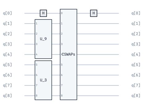
The SWAP test circuit is commonly used to evaluate the square of the modulus of an inner product. To obtain the SWAPTest circuit, we can simply use the SWAPTestBlock object.

This block takes the following arguments: bra - the bra preparation unitary, ket - the ket preparation unitary and (optional) measure - whether to measure the ancilla. Note, however, the preferred way to use measurement in OpenQARP is via a ReadoutBlock, or via Primitives. An example implementation is:

from qarp.blocks import ComputationalBasisStateBlock, SWAPTestBlock

u0 = ComputationalBasisStateBlock([1, 1, 0, 0]).build()
u1 = ComputationalBasisStateBlock([1, 0, 0, 1]).build()
swap = SWAPTestBlock(bra=u0, ket=u1).build()

SynthesizedTimeEvolutionBlock

The SynthesizedTimeEvolutionBlock creates a quantum circuit that implements exact time evolution under a Hamiltonian operator. Unlike TrotterBlock which approximates time evolution (\(\exp(-iHt)\)) using Trotterization, this block synthesizes the exact unitary by computing the matrix exponential and then decomposing it into quantum gates using our in-house Quantum Shannon Decomposition implementation.

Mathematical Background:

Given a Hamiltonian operator \(H\) and time parameter \(t\), the block implements:

\[U(t) = \exp(-iHt)\]

This is the exact time-evolution operator without Trotter approximation errors.

When to Use:

• High precision required: When Trotter errors are unacceptable

• Small systems: Works best for systems with few qubits (≤ 5-6 qubits) due to exponential circuit depth scaling

• Benchmarking: To compare against Trotterized circuits and assess Trotter error

• QMEGS and similar algorithms: When exact time evolution is needed for eigenvalue estimation

Required Arguments:

• operator: The Hamiltonian as a QubitOperator (must be Hermitian)

• n_qubits: Number of qubits the operator acts on

Optional Arguments:

• time: Evolution time parameter \(t\). Can be set during initialization or later via set_time()

• target_qubits: Indices of qubits to apply the evolution to (default: [0, 1, ..., n_qubits-1])

• name: Custom name for the block (default: "SynthTimeEvoBlock")

Example 1: Basic Time Evolution

from qarp.operators import QubitOperator
from qarp.blocks import SynthesizedTimeEvolutionBlock

# Define a simple Hamiltonian
hamiltonian = QubitOperator("Z0 X1") + QubitOperator("Y0 Y1")

# Create the time evolution block
time_evo = SynthesizedTimeEvolutionBlock(
    operator=hamiltonian,
    n_qubits=2,
    time=0.5
).build()

# Visualize the circuit
time_evo.plot()

Example 2: Dynamic Time Parameter

The time parameter can be set or updated after initialization, which is useful when you need to evaluate the same Hamiltonian at multiple time points:

from qarp.operators import QubitOperator
from qarp.blocks import SynthesizedTimeEvolutionBlock

hamiltonian = QubitOperator("Z0", 1.0)

# Create block without specifying time
time_evo = SynthesizedTimeEvolutionBlock(
    operator=hamiltonian,
    n_qubits=1
)

# set_time() returns a new, rebuilt block rather than mutating in place —
# capture the return value.
time_evo = time_evo.set_time(0.5)

# Update to a different time (returns a freshly-rebuilt block again)
time_evo = time_evo.set_time(1.0)

# Get the unitary matrix
import qarpx as qx
unitary = qx.QarpSimulator().unitary_matrix(time_evo.flatten(), time_evo.n_qubits)

Example 3: Fermi-Hubbard Model Evolution

from qarp.operators import JordanWigner
from qarp.operators.models import fermi_hubbard
from qarp.blocks import SynthesizedTimeEvolutionBlock

# Create a Fermi-Hubbard Hamiltonian with a genuine hopping term (one site
# has none, since there is nowhere to hop to, and Trotter is then exact
# regardless of step count) — use two sites so the comparison below is
# non-trivial, and so the operator spans the four qubits used below.
fham = fermi_hubbard((2,), t=0.14, U=0.231)
qham = JordanWigner().encode_operator(fham)

# Build exact time evolution
exact_evo = SynthesizedTimeEvolutionBlock(
    operator=qham,
    n_qubits=4,
    time=5.0,
).build()

# Compare with Trotter approximation
from qarp.blocks import TrotterBlock
trotter_evo = TrotterBlock(
    n_qubits=4,
    operator=qham,
    steps=10,
    time=5.0
).build()

# Check error. Unitary synthesis (via qarpx's Quantum Shannon Decomposition)
# does not preserve global phase, so a direct matrix difference would be
# dominated by an arbitrary phase rather than the actual Trotter error.
# Use the (phase-invariant) process infidelity instead.
import numpy as np
import qarpx as qx
sim = qx.QarpSimulator()
exact_u = np.array(sim.unitary_matrix(exact_evo.flatten(), exact_evo.n_qubits))
trotter_u = np.array(sim.unitary_matrix(trotter_evo.flatten(), trotter_evo.n_qubits))
dim = exact_u.shape[0]
fidelity = np.abs(np.trace(exact_u.conj().T @ trotter_u)) / dim
print(f"Trotter infidelity (1 - process fidelity): {1 - fidelity:.6f}")

Global Phase:

SynthesizedTimeEvolutionBlock synthesizes the circuit via qarpx’s Quantum Shannon Decomposition, which targets the exact unitary only up to a global phase (global phase has no physical effect on measurement statistics, so the synthesis routine does not track it). When comparing a synthesized circuit’s unitary against another one directly, use a global-phase-invariant metric such as process fidelity (\(|\mathrm{Tr}(U_1^\dagger U_2)| / d\)), as in the example above, rather than a raw matrix norm.

Performance Considerations:

• Circuit depth: Scales exponentially with number of qubits due to unitary synthesis

• Build time: Matrix exponentiation and synthesis can be slow for larger systems

• Use cases: Best suited for small systems (≤ 6 qubits) or when exact evolution is critical

• Alternative: Use TrotterBlock for larger systems where approximation is acceptable

Note

The operator must be Hermitian (as required for physical time evolution). The block validates this during initialization and raises a ValueError if the operator is non-Hermitian.

Warning

While this block provides exact time evolution without Trotter error, the resulting circuit depth grows exponentially with the number of qubits. For systems with more than 5-6 qubits, TrotterBlock is typically more practical despite the approximation error.

SynthesizedUnitaryBlock

The SynthesizedUnitaryBlock is a block which can create an arbitrary unitary, \(U\), as a block to act in a circuit. This is a very useful primitive for research purposes, for example we can use it to generate random unitaries in a circuit. However, care should be taken when using this block as it will lead to exponentially deep circuits in the number of qubits, since it makes no assumptions about the structure of the unitary.

It takes as its main argument unitary_matrix - the unitary matrix to synthesize (the synthesized circuit matches it up to a global phase; see the note above on comparing synthesized unitaries). An example implementation is as follows:

from scipy.stats import unitary_group
from qarp.blocks import SynthesizedUnitaryBlock

random_unitary = unitary_group.rvs(2**2)
print(random_unitary)

unitary_block = SynthesizedUnitaryBlock(random_unitary).build()

import qarpx as qx
circuit_unitary = qx.QarpSimulator().unitary_matrix(unitary_block.flatten(), unitary_block.n_qubits)
print(circuit_unitary)

unitary_block.plot()

Trotter Block

TrotterBlock implements the Suzuki-Trotter decomposition of the exponent of a Hamiltonian. Given a general Hamiltonian written as a sum of Pauli strings:

\[\begin{split}H = \sum^N_i \theta_i P_i, \\\end{split}\]

the exponent can be approximated using the Suzuki-Trotter approximation as:

\[\exp(-iHt) \approx \left( \exp\left(-i \theta_0 P_0 \frac{t}{M}\right) \exp\left(-i \theta_1 P_1 \frac{t}{M}\right) \cdots \exp\left(-i \theta_N P_N \frac{t}{M}\right)\right)^M.\]

TrotterBlock requires n_qubits - number of qubits and operator - the Hamiltonian to Trotterise as inputs. Additional optional inputs are: steps - number of Trotter steps, time - length of time evolution (can be a float or a sympy.Symbol for parametric circuits), order - order of expansion (must be 1 or even integer), grouping - a GroupingStrategy partitioning terms into sets that are exponentiated together (default FullyCommuting(); use NoGrouping() for the termwise circuit) and imaginary - whether to use the imaginary part of operator coefficients (True) or not (False).

An example implementation which trotterises and constructs the exponential of the Fermi-Hubbard chain Hamiltonian is as follows:

from qarp.operators import JordanWigner
from qarp.operators.models import fermi_hubbard
from qarp.blocks import TrotterBlock

fham = fermi_hubbard((2,), t=0.14, U=0.231)
qham = JordanWigner().encode_operator(fham)

trotter = TrotterBlock(n_qubits=4, operator=qham, steps=1, time=1.)

Note

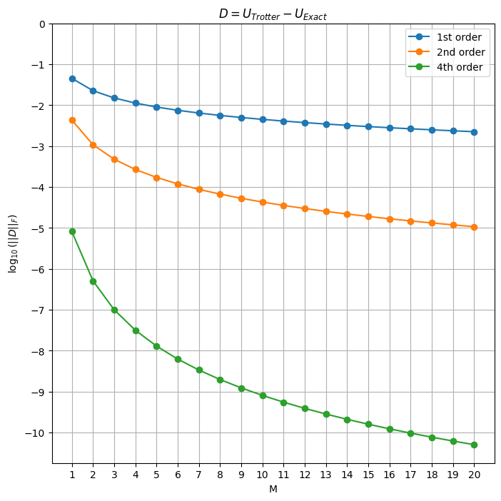
It is worth noting that while most applications of the Suzuki-Trotter approximation are limited to one step, this is still an approximation and only in the limit of infinitely many steps it becomes exact. However, we can easily increase the number of Trotter steps in OpenQARP by changing the step argument in the constructor.

To see how the Trotter error scales for this example with the number of steps, see the log-plot below.

Symbolic Time Parameter

TrotterBlock supports symbolic time parameters using sympy.Symbol. This is useful when you want to build a parametric circuit where the evolution time can be substituted later without rebuilding the circuit. To substitute the time value, use the set_time() method, which handles the internal \(\pi\) normalization correctly.

from sympy import Symbol
from qarp.operators import JordanWigner
from qarp.operators.models import fermi_hubbard
from qarp.blocks import TrotterBlock

fham = fermi_hubbard((2,), t=0.14, U=0.231)
qham = JordanWigner().encode_operator(fham)

# Create a symbolic time parameter
t = Symbol("t")
trotter = TrotterBlock(n_qubits=4, operator=qham, steps=1, time=t).build()

# The block now contains the symbolic parameter. `.symbols` is a sorted
# tuple (see the note on Block.symbols above), not a set.
print(trotter.symbols)  # (t,)

# Substitute the time value using set_time()
trotter_t1 = trotter.set_time(1.0)
trotter_t05 = trotter.set_time(0.5)

# The substituted blocks no longer contain the symbol
print(trotter_t1.symbols)  # ()

# Plot the circuit
trotter.plot(scrollable=True)
trotter_t05.plot(scrollable=True)
trotter_t1.plot(scrollable=True)

Warning

When substituting time values, prefer the set_time() method over the generic set_symbols() method. set_time() is a thin wrapper that calls set_symbols() with the block’s internal time symbol; using set_symbols() directly works but you must reference the same Symbol instance the block was built with.

Trotter Ansatz Block

TrotterAnsatzBlock constructs a parametric Trotterized circuit from a list of qubit operators and their associated symbols. Unlike TrotterBlock which takes a fixed operator, TrotterAnsatzBlock allows each term in the Hamiltonian to have its own variational parameter, making it suitable for variational quantum algorithms like VQE.

This block requires the following arguments:

• n_qubits: The number of qubits the circuit acts on.

• qubit_exponents: A list of QubitOperator objects representing the terms in the ansatz.

• symbols: A list of sympy.Symbol objects, one for each qubit exponent.

Optional arguments include: steps - number of Trotter steps, time - global time scaling factor (can be a float or sympy.Symbol), order - order of the Trotter expansion (must be 1 or even integer), grouping - the GroupingStrategy used to partition terms into commuting sets, and imaginary - whether to use the imaginary part of operator coefficients.

Grouping is applied within each (symbol, operator) pair, never across them: the ansatz is the ordered product ∏_k exp(θ_k G_k), so the generator order is meaningful and must not be permuted. Since a generator’s own Pauli terms commute, each generator is emitted as a single exact exponential.

An example implementation using the UCC ansatz operators:

from sympy import Symbol
from qarp.blocks import TrotterAnsatzBlock
from qarp.operators import JordanWigner, NoGrouping
from qarp.operators.ucc import ucc_singles_and_doubles

# Generate UCC operators
onv = [1, 1, 0, 0]
uccsd, symbols = ucc_singles_and_doubles(onv, spin_conserving=True, generalised=False)
quccsd = JordanWigner().encode_operator(uccsd)

# Build the ansatz block
ansatz = TrotterAnsatzBlock(
    n_qubits=4,
    qubit_exponents=quccsd,
    symbols=symbols,
    steps=1,
    order=1,
    grouping=NoGrouping(),
    imaginary=True,
).build()

# Substitute parameter values
param_map = {s: 0.1 * i for i, s in enumerate(symbols)}
ansatz_substituted = ansatz.set_symbols(param_map)

# Plot the circuit
ansatz.plot(scrollable=True)
ansatz_substituted.plot(scrollable=True)

A single-generator instance (for illustration) keeps the circuit small enough to show in full:

from sympy import Symbol
from qarp.blocks import TrotterAnsatzBlock
from qarp.operators import QubitOperator

theta = Symbol("theta")
small_ansatz = TrotterAnsatzBlock(
    n_qubits=2, qubit_exponents=[QubitOperator("Y0 X1", 1.0)], symbols=[theta]
).build()

Symbolic Time in TrotterAnsatzBlock

Similar to TrotterBlock, the TrotterAnsatzBlock also supports symbolic time parameters. When the time argument is a sympy.Symbol, the time symbol is automatically added to the block’s symbol list. Use the set_time() method to substitute the time value:

from sympy import Symbol
from qarp.blocks import TrotterAnsatzBlock
from qarp.operators import JordanWigner
from qarp.operators.ucc import ucc_singles_and_doubles

onv = [1, 1, 0, 0]
uccsd, symbols = ucc_singles_and_doubles(onv, spin_conserving=True, generalised=False)
quccsd = JordanWigner().encode_operator(uccsd)

# Create with symbolic time
t = Symbol("t")
ansatz = TrotterAnsatzBlock(
    n_qubits=4,
    qubit_exponents=quccsd,
    symbols=symbols,
    time=t,  # Symbolic time parameter
    imaginary=True,
).build()

# The time symbol joins the block's symbols
print(t in ansatz.symbols)  # True

# Substitute time using set_time()
ansatz_evolved = ansatz.set_time(0.5)

# Other parameters can still be substituted separately
param_map = {s: 0.1 for s in symbols}
ansatz_final = ansatz_evolved.set_symbols(param_map)

# Plot the circuit
ansatz.plot(scrollable=True)
ansatz_evolved.plot(scrollable=True)
ansatz_final.plot(scrollable=True)

Unitary Coupled Cluster Block

The UCCBlock constructs a parameterized quantum circuit representing the UCC ansatz, which approximates the electronic structure wavefunction through exponentials of particle-hole excitation operators. The block generates single and/or double excitations from a reference occupation, transforms them to qubit operators via fermion-to-qubit mappings, and implements the unitary via Trotterization. This provides a chemically-inspired ansatz for VQE that respects particle number and spin symmetries.

This block requires the argument occupation_number_vector - occupation number vector defining the initial state (a plain abab list of 0s and 1s), and takes the following optional arguments: singles - whether to include single excitation operators, doubles - whether to include double excitation operators, paired_doubles - whether to restrict doubles to paired excitations, generalised - whether to use generalized excitation operators, spin_conserving - if True, only includes spin-conserving excitations, mapping - Fermion-to-qubit mapping (default: Jordan-Wigner), order - Trotter decomposition order, time - evolution time parameter, steps - number of Trotter steps and grouping - the GroupingStrategy forwarded to the inner TrotterAnsatzBlock.

For example, to construct the block representing the UCCSD unitary:

from qarp.blocks import UCCBlock
from qarp.operators import JordanWigner

onv = [1, 1, 0, 0]
ucc = UCCBlock(occupation_number_vector=onv, mapping=JordanWigner(), singles=True, doubles=True, generalised=False)
ucc.build()

To construct the generalised UCCSD unitary, set the generalised flag to True.

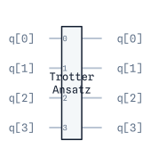
Note

The reference state is not encoded on the circuit! Only the UCC portion is added to the block. This is to simplify usage with some of the algorithms. To include the reference state, first generate the UCCBlock similarly to above, then use something like my_ansatz = CompositeBlock([MappedONVStateBlock(onv, JordanWigner()).build(), ucc]).build().

Xn Block

XnBlock applies an X gate to each of the qubits, flipping them all to the \(|1\rangle\) state.

It takes n_qubits - number of qubits as an input.

An implementation is as follows:

from qarp.blocks import XnBlock

n_qubits = 4
block = XnBlock(n_qubits=n_qubits).build()

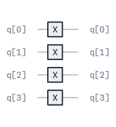
Yoshida-Trotter composition

TrotterBlock supports Trotterization at orders 6 and 8 at significantly lower depth than its default "suzuki" recursion, via composition="yoshida". For details of 6th order Trotter see this publication by Yoshida et al. For 8th order Trotter, see this publication by Morales et al.

To construct a Yoshida-composed TrotterBlock:

from qarp.operators import JordanWigner
from qarp.operators.models import fermi_hubbard
from qarp.blocks import TrotterBlock

# A single Fermi-Hubbard site (two spin orbitals) keeps the order-6
# expansion small enough to read; the composition is the point, not the
# system size.
fham = fermi_hubbard((1,), t=0.14, U=0.231)
qham = JordanWigner().encode_operator(fham)

trotter = TrotterBlock(n_qubits=2, operator=qham, steps=1, time=1.0, order=6, composition="yoshida")

Tensor Network Blocks

VUMPO Brickwork Block

The VUMPOBrickworkBlock implements a brickwork‑structured layer of the Variational Unitary Matrix Product Operator (VUMPO) ansatz, introduced by Pollmann et al. in Efficient variational diagonalization of fully many-body localized Hamiltonians, Phys. Rev. B 94, 041116(R) (2016), https://doi.org/10.1103/PhysRevB.94.041116.

A VUMPO layer consists of alternating even‑ and odd‑indexed two qubit unitaries arranged in a brickwork pattern. Each gate is generated via the internal parameterization of a VUMPO object, representing a low bond dimension unitary tensor network operator. If optimal parameters are not passed, the block builds the vumpo (via vumpo.build()) internally before splitting into gates and applies the resulting two qubit unitaries to qubit pairs \((n, n+1)\) with offset \(m % 2\) for layer \(m\).

Optionally, an initial computational basis state block may be prepended when an initial_state is supplied, enabling computational basis state preparation before the variational brickwork layers.

See qarp.operators.VUMPO for more details on the actual VUMPO tensor networks construction.

The two qubit unitaries come out of quimb in the opposite qubit ordering to qarpx, so the block conjugates each one with a two qubit SWAP before applying it (see Endianness). That conversion is what makes the circuit act on the register qarpx actually uses; without it the layer silently acts on the wrong qubit ordering.

Both VUMPO and VUMPOBrickworkBlock need the [mps] extra (quimb) installed.

An example VUMPO configuration (for illustration) is shown below:

import numpy as np
from qarp.blocks import VUMPOBrickworkBlock
from qarp.operators import VUMPO
from quimb.tensor import MatrixProductOperator

L = 4
rng = np.random.default_rng(0)   # seeded so the circuit below is reproducible

A = (rng.standard_normal((2**L, 2**L)) + 1j*rng.standard_normal((2**L, 2**L)))
ham_mat = (A + A.conj().T) / 2
# quimb's from_dense is kron-ordered (site 0 = leftmost factor = qubit L-1 of a
# qarpx-LSB matrix); VUMPO puts site n on qubit n.  A random matrix has no
# qubit meaning, so no reversal is needed here — for an operator matrix use
# from_dense(lsb_to_msb_matrix(op.sparse_matrix().toarray()), ...).
H_mpo = MatrixProductOperator.from_dense(ham_mat, dims=(2,)*L)

vumpo = VUMPO(
      H_mpo=H_mpo,
      n_layers=3,
      n_sweeps=2,
      maxiter_local=2,
      mode="diag",
      opt="local",
)
initial_state = np.array([1] * (2) + [0] * (2))

params = vumpo.build()
vumpo_block = VUMPOBrickworkBlock(
   vumpo=vumpo, initial_state=initial_state, optimized_params=params
)
vumpo_block.build()

The resulting brickwork circuit, with the basis-state preparation prepended:

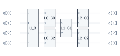
State preparation

State-preparation blocks define circuits encoding initial wavefunctions for certain algorithms.

Declaring the prepared state

A primitive is specified by its whole unitary; a block that prepares a state is specified by a single column of it, \(U|0\ldots0\rangle\), with the remaining columns free. AmplitudeAmplificationBlock shows why: \(Q = A S_0 A^\dagger S_\chi\) is correct for any unitary \(A\) whose zeroth column is \(|\psi\rangle\), since \(A S_0 A^\dagger = 2|\psi\rangle\langle\psi| - I\) no matter what the other columns hold. Two blocks preparing the same state can therefore have entirely different matrices and both be right, so there is no unitary oracle to test them against.

PreparesKnownState is that column, declared. Attach it with the prepares_known_state decorator:

from qarp.blocks import SimpleBlock, prepares_known_state

@prepares_known_state
class MyStateBlock(SimpleBlock):
    def build_vanilla(self):
        ...

    def target_statevector(self):
        """The state this block leaves on |0…0⟩ — derived from the maths, not the circuit."""
        ...

The declaration carries six members:

state_qubits

Block-local indices carrying the prepared state, ascending. Defaults to the whole register; override it when the block sizes itself larger than the state it prepares, as the QRAM blocks do — CVOQRAMStateBlock reports n_qubits = 2n but prepares an \(n\)-qubit state.

ancilla_qubits

The complement, derived.

ancilla_postselection

The condition under which the prepared state appears, as a PostSelection, or None. None means every ancilla returns to \(|0\rangle\) with probability 1 — the block is deterministic and safe under ControlledBlock. A returned condition means the state exists only on that branch; hand it straight to a Sampler result.

target_statevector()

The declared state, 2**len(state_qubits) amplitudes, LSB, including global phase. Standalone a global phase is unobservable, but under ControlledBlock it becomes a physical relative phase — and AmplitudeEstimationBlock controls its state-preparation block.

is_exact

True by default: the built circuit is asserted to match target_statevector() exactly (elementwise, atol=1e-10). Override to False for a block whose construction is inherently approximate — a fixed-precision discretization, a truncated low-rank/MPS expansion — alongside error_bound.

error_bound

Upper bound on 1 - |⟨target|prepared⟩|² (infidelity); only meaningful when is_exact is False, in which case the conformance suite checks infidelity against this bound instead of exact equality. Should be computable from the block’s own construction (a discarded Schmidt weight, a discretization precision), not fitted after the fact.

The counterpart prepared_statevector() returns what the built circuit actually leaves, together with the probability of the declared condition, so the two can be compared directly:

from qarp.blocks import CVOQRAMStateBlock
import numpy as np

block = CVOQRAMStateBlock({(1, 0, 1): 0.6, (0, 1, 0): -0.8}).build()

block.n_qubits                  # 6 — the block's full register
block.state_qubits              # (3, 4, 5) — only these carry the state
block.ancilla_postselection     # None: the ancillas are restored, so it is control-safe

prepared, probability = block.prepared_statevector()
np.allclose(prepared, block.target_statevector())   # True, phase included

Declaring is opt-in and independent of where a block lives: a leaf SimpleBlock and a CompositeBlockBase tree declare it the same way. Parameterized ansätze must not — UCCBlock, HEABlock, SPABlock and QAOABlock have no fixed column, because their output depends on symbol values and on the reference state they are applied to. declaring_blocks() lists every block that has declared it.

One limit worth stating plainly: the declaration is checked against the circuit, not proved correct by it. A target_statevector() that is wrong in the same way as the circuit passes that check. The independent oracle (§18) remains a per-block obligation.

Computational Basis State

The ComputationalBasisStateBlock is a simple circuit that prepares a specific basis state on a given set of qubits. It simply is a sequence of X gates applied to the qubits that are set to 1 in basis_state.

It requires input basis_state - a list of 0s and 1s representing the basis state to prepare, LSB-first: entry q is qubit q, not a binary literal (see Endianness).

The syntax to apply the Basis State block in OpenQARP is as follows:

from qarp.blocks import ComputationalBasisStateBlock

n_qubits = 4
state = [1, 1, 0, 0]  # qubits 0 and 1 occupied -> X on each
basis_state_block = ComputationalBasisStateBlock(state, target_qubits=list(range(n_qubits))).build()

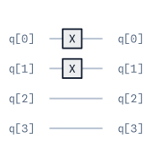
CV-QRAM and CVO-QRAM Block

This Block implements CV-QRAM and CVO-QRAM (de Veras, T. M. et al. (2022) Quantum Information Processing) state preparation method, where the latter is an improved version of the former in which the number of 2-qubit gates are drastically reduced.

This block takes the argument dataset - a dictionary specifying the data to be loaded with tuples as keys and amplitudes as values.

An example implementation is as follows:

from qarp.blocks import CVOQRAMStateBlock
import numpy as np

dataset = {(1, 0, 0): np.sqrt(0.5), (0, 0, 0): np.sqrt(0.5)}

cvoqram_block = CVOQRAMStateBlock(dataset, target_qubits=list(range(6))).build()
cvoqram_block.plot()

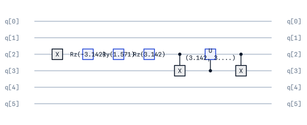
Dicke State

The DickeStateBlock prepares a superposition of all basis states with a given Hamming weight. It is useful, for example, for preparing states with a fixed number of fermions under the Jordan-Wigner mapping, such as in quantum-chemistry applications.

It requires inputs n_qubits - number of qubits and hamming_weight- the Hamming weight of each term in the dicke state.

We use the method of Bärtschi, A., Eidenbenz, S. - Fundamentals of Computation Theory. FCT 2019, vol 11651

An example of a Dicke state on \(4\) qubits in a Hamming weight \(2\) subspace

\[|\psi\rangle = \frac{1}{\sqrt{\binom{4}{2}}}\left(|1100\rangle + |1010\rangle + |1001\rangle + |0110\rangle + |0101\rangle + |0011\rangle\right)\]

from qarp.blocks import DickeStateBlock

# Create a Dicke state of 4 qubits with Hamming weight 2
# (that is, equal superposition of |1100⟩, |1010⟩, |1001⟩, |0110⟩, |0101⟩, |0011⟩)
dicke_block = DickeStateBlock(n_qubits=4, hamming_weight=2).build()
dicke_block.plot()

GHZ Like State

The GHZLikeStateBlock prepares a multi-qubit entangled state resembling a GHZ state but localized to specific basis states. It creates entanglement by applying a Hadamard gate to the first qubit marked as \(|1\rangle\) in the basis state, then cascading CNOT gates to entangle subsequent \(|1\rangle\)-marked qubits.

It requires arguments basis_state - a list of 0s and 1s representing which qubits participate in the GHZ-like state, and dephase - if True, applies \(S^{\dagger}\) gate to introduce phase factor \(i\) in the superposition.

The GHZ states are maximally-entangled quantum states defined for \(N\) qubits as

\[|\rm{GHZ}\rangle = \frac{1}{\sqrt{2}} (|0\rangle^{\otimes N} + |1\rangle^{\otimes N})\]

A GHZ-like state is a similar \(N\)-qubits state but maximally-entangled only in a subset of the qubits. For example,

\[|000\rangle + |101\rangle\]

is a GHZ-like state for the first and third qubits.

An example implementation is as follows:

from qarp.blocks import GHZLikeStateBlock

state = [1, 1, 0, 1]
ghz_like_block = GHZLikeStateBlock(state).build()

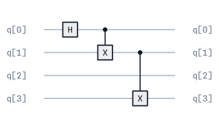
Hypergraph State

HypergraphStateBlock prepares quantum states defined by hypergraphs, where vertices represent qubits and hyperedges encode multi-qubit entangling operations. Starting from an equal superposition (\(H^{\otimes n}|0\rangle^{\otimes n}\)), controlled-Z gates are applied according to the hypergraph structure, creating states with higher-order correlations beyond pairwise entanglement.

This block takes as arguments hypergraph - a Hypergraph object defining the state structure, n_qubits - number of qubits and edges - list of hyperedges, each a tuple of qubit indices. Either hypergraph or both n_qubits and edges must be provided. An example implementation is as follows:

from qarp.blocks import HypergraphStateBlock
import hypernetx as hnx

edges = [(1, 2), (2, 3), (1, 2, 3)]

HPG = hnx.Hypergraph(edges)
hnx.draw(HPG)

block = HypergraphStateBlock(edges=edges, n_qubits=4).build()
block.plot()

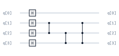
On this edges path the block’s hypergraph attribute is the equivalent Hypergraph when the [hypergraph] extra is installed and None otherwise; the block itself does not need hypernetx. The graph types build it for you: Hypergraph.to_state_block() and, for a graph state (order-2 hyperedges only), Graph.to_graph_state_block() — see Graphs.

The block can also take a OpenQARP Hypergraph object directly. For more detail on OpenQARP Hypergraphs see qarp.graphs.Hypergraph. When constructing the Hypergraph this way, vertex labels must be non-negative integers (qubit indices); n_qubits is inferred as the highest vertex index plus one, so a sparse labelling (e.g. skipping a qubit index, as vertex 4 is skipped below) still reserves every qubit up to the highest one used.

import hypernetx as hnx

from qarp.blocks import HypergraphStateBlock
from qarp.graphs import Hypergraph

edges = {
   "e0": [0, 1, 2],
   "e1": [2, 3],
   "e2": [2, 3, 5],
   "e3": [0, 6],
}

HPG = Hypergraph(edges)
hnx.draw(HPG)

block = HypergraphStateBlock(hypergraph=HPG).build()
block.plot()

Mapped Onv State

MappedONVStateBlock prepares the basis state corresponding to the input occupation number vector given a mapping.

This block takes as arguments occupation_number_vector - the ONV in Fock space and mapping - the mapping to use to obtain the relevant basis state. An example implementation is as follows:

from qarp.blocks import MappedONVStateBlock
from qarp.operators import JordanWigner

onv = [1, 1, 0, 0]
MappedONVStateBlock(occupation_number_vector=onv, mapping=JordanWigner())

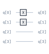
Synthesized State

SynthesizedStateBlock prepares an arbitrary quantum state defined by a set of amplitudes. Note, care should be taken as this is a method for _generic_ state preparation - in general the circuit will have exponentially many gates and depth.

This block takes the arguments n_qubits - number of qubits and amplitudes - amplitudes defining the quantum state, either a list for all basis states or a dictionary mapping basis state tuples to complex amplitudes.

For example, we can prepare the uniform superposition state on two qubits as follows:

\[|\psi\rangle = \frac{1}{\sqrt{2^2}} \left(|00\rangle + |01\rangle + |10 \rangle + |11\rangle \right)\]

import numpy as np
from qarp.blocks import SynthesizedStateBlock

amps = np.array([1 / np.sqrt(4), 1 / np.sqrt(4), 1 / np.sqrt(4), 1 / np.sqrt(4)])
state_block = SynthesizedStateBlock(2, amps)

To be a valid quantum state, the amplitudes should be normalised. If amplitudes are passed which are not normalised, the block also normalised them before preparing. For example, with the below state.

from qarp.blocks import SynthesizedStateBlock

amps = [0.1 + 0.2j, 0, 0, 0.2 + 0.1j]
state_block = SynthesizedStateBlock(2, amps).build()

import qarpx as qx
print(qx.QarpSimulator().statevector(state_block.flatten(), state_block.n_qubits))

We can also pass a dictionary of amplitudes as follows. Basis-state tuples are written qubit-``n_qubits-1`` first, qubit-0 last (like a bitstring literal, e.g. "q1 q0" for 2 qubits) — the last tuple entry is qubit 0, which is the least-significant index in the qarpx command-level convention. For example, (0, 1) (qubit 1 = 0, qubit 0 = 1) and (1, 1) and (0, 0) below reproduce the same two basis states as the list-based example above, since only the symmetric (0, 0)/(1, 1) entries are populated:

amps = [0.1 + 0.2j, 0, 0, 0.2 + 0.1j]
norm_amps = sum(abs(a) ** 2 for a in amps) ** 0.5

amps_dict = {(0, 0): (0.1 + 0.2j) / norm_amps, (0, 1): 0, (1, 0): 0, (1, 1): (0.2 + 0.1j) / norm_amps}
state_block = SynthesizedStateBlock(2, amps_dict).build()

print(qx.QarpSimulator().statevector(state_block.flatten(), state_block.n_qubits))

Sparse State

SparseStateBlock prepares a state given by only a handful of nonzero amplitudes, ancilla-free. Unlike SynthesizedStateBlock, which builds every one of the \(2^n\) computational-basis branches regardless of how many are actually populated, this block only builds gates for the branches its s nonzero amplitudes touch — and unlike CVQRAMStateBlock / CVOQRAMStateBlock, it does not widen the register with ancilla qubits. It cites Gleinig & Hoefler (DAC 2021) and Malvetti, Iten & Colbeck (Quantum 5, 412 (2021)) for the ancilla-free \(O(s\,n)\)-CNOT merge procedure, which it does not yet implement.

Cost, measured as CNOTs after decomposition on clifford_t_rz_gateset at O0: each multi-controlled rotation is a Barenco cascade over an ancilla-free mcx, so the total scales as roughly \(O(s\,n^4)\). For \(s = 2\) it is 500 CNOTs at \(n = 6\) (dense SynthesizedStateBlock: 124), 9 908 at \(n = 10\) (≈ 2 048), 118 274 at \(n = 16\) (≈ 131 072 — the crossover, ratio 0.90), 262 516 at \(n = 20\) (ratio 0.13) and 568 098 at \(n = 24\) (ratio 0.02). Below \(n \approx 16\) it is therefore more expensive than dense synthesis and only wins above; the cited merge would need ≈ 100 CNOTs at \(n = 16, s = 2\). The rewrite to that construction is a declared follow-up.

This block takes the arguments n_qubits and amplitudes — a dictionary mapping basis-state tuples (LSB-first, tuple element i is qubit i, §1) to complex amplitudes. Unlisted basis states are implicitly zero; listed amplitudes are normalised internally, and entries whose normalised modulus is below 1e-15 are dropped.

from qarp.blocks import SparseStateBlock

amplitudes = {
    (1, 0, 0): 1 / np.sqrt(2),
    (0, 1, 1): 1 / np.sqrt(2),
}
state_block = SparseStateBlock(3, amplitudes).build()

import qarpx as qx
print(qx.QarpSimulator().statevector(state_block.flatten(), state_block.n_qubits))

Multi-ONV State

MultiONVStateBlock generalises MappedONVStateBlock from a single occupation-number vector to a superposition of several — a CI-vector reference (e.g. a CASCI or CISD ground state) rather than a single Hartree-Fock determinant, for use as a QPE or ADAPT reference state. Each ONV is mapped independently through the given mapping (default JordanWigner()), and the resulting basis states are loaded with the same ancilla-free construction as SparseStateBlock — so the cost is SparseStateBlock’s, with s the number of determinants (see the measured numbers and the declared follow-up there). Under Bravyi–Kitaev pass BravyiKitaev(n_qubits=len(onv)) so the operator transform and encode_state agree on the register width.

The determinant sign convention: the coefficient of ONV b multiplies \(a^\dagger_{p_1} a^\dagger_{p_2} \cdots a^\dagger_{p_k}|\text{vac}\rangle\) with \(p_1 < p_2 < \cdots < p_k\) the occupied spin-orbital indices in abab order (2·spatial for α, +1 for β) — exactly what products of FermionOperator creation operators give.

This block takes onv_coefficients — a dictionary mapping occupation-number vectors (as tuples of 0/1, abab order) to complex CI coefficients — and an optional mapping.

from qarp.blocks import MultiONVStateBlock
from qarp.operators import JordanWigner

onv_coefficients = {
    (1, 1, 0, 0): 0.6,
    (1, 0, 0, 1): 0.8,
}
state_block = MultiONVStateBlock(onv_coefficients, mapping=JordanWigner()).build()

pyscf CI vectors use an αα…ββ… string order that needs a per-determinant sign to reach this convention; qarp.operators.pyscf.onv_coefficients_from_civec() applies it (see Operators). pyscf is optional and imported lazily:

from pyscf import fci, gto, scf
from qarp.operators.pyscf import onv_coefficients_from_civec

mf = scf.RHF(gto.M(atom="H 0 0 0; H 0 0 1.5", basis="sto3g")).run()
energy, civec = fci.FCI(mf).kernel()
state_block = MultiONVStateBlock(onv_coefficients_from_civec(civec, 2, mf.mol.nelec)).build()

Slater Determinant

SlaterDeterminantBlock prepares a Slater determinant of orbitals that are a rotation of the qubit orbitals, exact and ancilla-free — a Givens-rotation network (Kivlichan et al., PRL 120, 110501 (2018); Jiang et al., PR Applied 9, 044036 (2018)) built on top of the existing GivensBlock / OrbitalRotationBlock. In the qubit basis this is a superposition of up to \(\binom{N}{M}\) occupation-number states — the natural-orbital or localised-orbital reference that MappedONVStateBlock cannot express. When the two bases coincide (Q a slice of the identity up to column order and signs) the state is a single ONV: use MappedONVStateBlock, or rely on this block’s short-circuit, which then emits only the X layer (plus a gphase(π) when the signed permutation is odd, so the declared phase is kept exactly).

This block takes orbital_coefficients — a real (n_modes, n_occupied) matrix Q with orthonormal columns, describing \(b^\dagger_1 \cdots b^\dagger_M |\text{vac}\rangle\) where \(b^\dagger_i = \sum_p Q_{pi} a^\dagger_p\). Mode p is qubit p under Jordan-Wigner, the same convention OrbitalRotationBlock uses, and rows of Q are spin orbitals in abab order (§1): row 2·spatial is the α spin orbital, row 2·spatial + 1 its β. An RHF caller holding a spatial matrix interleaves it themselves — each occupied spatial column becomes an α column on the even rows and a β column on the odd rows; a (C_alpha, C_beta) spatial-blocks constructor is a declared follow-up. Q is accepted to \(\|Q^T Q - I\| \le 10^{-8}\) and re-orthonormalised. Complex orbital coefficients are not supported — GivensBlock has no phase parameter.

Cost (measured): the block completes Q to a full orthogonal U and applies the \(N(N-1)/2\) Givens QR of OrbitalRotationBlock — 22 Givens rotations, 88 CNOTs on clifford_t_rz_gateset, at \(N = 8, M = 4\), against Kivlichan’s \(M(N-M) = 16\) bound. Within a factor 1.4 of optimal; the rectangular decomposition is the other declared follow-up in the plan.

from qarp.blocks import SlaterDeterminantBlock
import numpy as np

# Any real matrix with orthonormal columns — e.g. from a QR decomposition
# of the occupied-orbital block of a Hartree-Fock coefficient matrix.
orbital_coefficients, _ = np.linalg.qr(np.random.default_rng(0).normal(size=(4, 4)))
state_block = SlaterDeterminantBlock(orbital_coefficients[:, :2]).build()

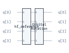
CSF (Spin-Adapted) State

CSFStateBlock prepares a configuration state function directly, exact and ancilla-free — unlike the LCU projector blocks above (SzProjectorBlock / SpinSquaredProjectorBlock, which succeed only with some probability), this builds the target linear combination of determinants classically (via the genealogical/Yamanouchi-Kotani spin-coupling scheme, using sympy.physics.quantum.cg.CG()) and loads it deterministically with MultiONVStateBlock — no postselection.

This block takes n_spatial_orbitals, core_orbitals (doubly occupied), open_shell_orbitals (singly occupied, in coupling order), Ms, and exactly one of S (keyword-only, the total spin) or coupling_path (the intermediate total spins reached after coupling each open-shell electron in turn). S selects the canonical path — couple upwards by \(1/2\) at every step until the largest intermediate spin needed, then downwards to S: [1/2, 0] for the two-electron singlet, [1/2, 1, 1/2] for the three-electron doublet. For \(k \ge 3\) open-shell electrons more than one linearly independent CSF shares the same final S (two doublets for \(k = 3\), the allyl-radical case), and coupling_path picks a specific one — [1/2, 0, 1/2] is the other doublet.

The block emits every determinant with creation operators in ascending spin-orbital index (the MultiONVStateBlock convention), whereas the textbook CSF is written in coupling order; the two differ by the same permutation for every determinant, so a textbook CSF may appear with an overall \(-1\) while relative signs are unaffected.

Cost: the CSF expands into \(\binom{k}{k/2 + M_s}\) determinants — exponential in \(k\) — each riding the sparse-state construction above, so this is fine for \(k \le 6\) or so. A direct CSF circuit (Sugisaki et al., JCTC 2019: sequential spin-coupling gates, no determinant expansion) is the declared follow-up.

from qarp.blocks import CSFStateBlock

# The textbook 2-electron singlet: (|up down> - |down up>) / sqrt(2)
state_block = CSFStateBlock(
    n_spatial_orbitals=2,
    core_orbitals=[],
    open_shell_orbitals=[0, 1],
    S=0,
    Ms=0,
).build()

# Three open-shell electrons: two doublets share S = 1/2, so pick one by path
doublet = CSFStateBlock(
    n_spatial_orbitals=3,
    core_orbitals=[],
    open_shell_orbitals=[0, 1, 2],
    coupling_path=[0.5, 0, 0.5],
    Ms=0.5,
).build()

Decomposed into its underlying MultiONVStateBlock gates: the two-determinant singlet \((|{\uparrow\downarrow}\rangle - |{\downarrow\uparrow}\rangle)/\sqrt{2}\).

Low-Rank (Schmidt-Truncated) State

LowRankStateBlock is an ε-dial for SynthesizedStateBlock: it approximates an arbitrary dense state by truncating its Schmidt rank across a chosen qubit bipartition (Araujo et al., Sci. Rep. 11, 6329 (2021)). This is the first block to use the is_exact / error_bound members of PreparesKnownState (see “Declaring the prepared state” above): is_exact is True exactly when max_schmidt_rank is left at the full rank (the default), and error_bound is the discarded Schmidt weight, which is the exact infidelity to the un-truncated target, not merely an upper bound on it.

Cost, measured as CNOTs on clifford_t_rz_gateset at O0: truncation currently buys no circuit saving, because a full \(2^{\text{cut}} \times 2^{\text{cut}}\) unitary is synthesised per side. At \(n = 8, \text{cut} = 4\) rank 1 costs 336, rank 2 costs 337 and full rank 16 costs 568, against 508 for the dense SynthesizedStateBlock; at \(n = 6\) rank 1 costs 72, full rank 111, dense 124. Araujo’s saving comes from synthesising only the rank constrained columns (an isometry), and rank 1 should be two plain state preparations (≈ 30 CNOTs at \(n = 8\)); both are declared follow-ups. Until they land, use this block for the ε-dial, not for cost.

This block takes n_qubits, amplitudes (a dense list or dict, same convention as SynthesizedStateBlock), cut (splitting the register into A = [0, cut) and B = [cut, n) — defaults to the middle), and max_schmidt_rank (defaults to the full rank, i.e. exact reconstruction).

from qarp.blocks import LowRankStateBlock
import numpy as np

amplitudes = np.random.default_rng(0).normal(size=16) + 1j * np.random.default_rng(1).normal(size=16)
state_block = LowRankStateBlock(4, list(amplitudes), cut=2, max_schmidt_rank=2).build()

state_block.is_exact   # False: rank 2 of a full rank 4
print(f"infidelity to the exact target <= {state_block.error_bound:.4f}")

LowRankStateBlock(4, list(amplitudes), cut=2).build().is_exact   # True at the default (full) rank

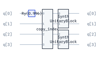
Matrix Product State

MPSStateBlock prepares a state given as an open-boundary matrix product state, exact — the “I ran DMRG, give me a circuit” case (Schön et al., PRL 95, 110503 (2005), “exact sequential”). Unlike VUMPOBrickworkBlock (a variational ansatz whose parameters are optimized against a target), this takes an already-known MPS and emits an exact circuit for whatever it represents; it needs no approximation dial, since a valid MPS reproduces exactly (any inaccuracy from how that MPS was obtained — a DMRG bond-dimension truncation, say — is a property of the input, not of the block). A bond register of \(\lceil\log_2\chi\rceil\) qubits threads through the chain and is returned to \(|0\ldots0\rangle\) deterministically by the trivial right boundary, so ancilla_postselection is None.

Cost, measured as CNOTs on clifford_t_rz_gateset at O0: this is the one block on this page whose measured cost already scales well — one \((2\chi) \times (2\chi)\) unitary per site, so linear in \(N\). For \(\chi = 2\) it is 24 at \(N = 4\) (dense SynthesizedStateBlock: 28), 36 at \(N = 6\) (124) and 48 at \(N = 8\) (508), plus the \(\lceil\log_2\chi\rceil\) bond-register ancillas. The ancilla-free sliding-window form (Ran, PRA 101, 032310 (2020)) removes those, and synthesising each site as an isometry rather than a full unitary trims the constant; both are declared follow-ups.

This block takes tensors — a list of site tensors, each of shape (chi_left, 2, chi_right), with chi_left = 1 for the first site and chi_right = 1 for the last (open boundary conditions). Site k maps to qubit k (LSB, §1). The tensors need not already be canonical or have minimal bond dimension.

Note

Converting from a third-party MPS library’s own tensors may need an endianness fix — quimb’s from_dense is kron/MSB-ordered (qarp/endianness.py), the opposite of this block’s LSB convention; reverse the site order and swap each tensor’s bond axes when converting.

from qarp.blocks import MPSStateBlock
import numpy as np

# 0.6|00> + 0.8|11>, as a 2-site MPS with bond dimension 2
tensors = [
    np.array([[[0.6, 0.0], [0.0, 0.8]]]),
    np.array([[[1.0], [0.0]], [[0.0], [1.0]]]),
]
state_block = MPSStateBlock(tensors).build()

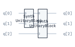
Uniform Superposition (Non-Power-of-Two)

UniformSuperpositionBlock prepares \(\frac{1}{\sqrt{M}}\sum_{j=0}^{M-1}|j\rangle\) for arbitrary integer M — not just a power of two — exact and ancilla-free, with \(L = \lceil\log_2 M\rceil\). Constantly needed for constrained QAOA, counting, and non-power-of-two lattices. It cites Shukla & Vedula, Quantum Inf. Process. 23, 38 (2024), whose Algorithm 1 costs \(O(L)\) single-control gates — which this block does not yet implement: it writes M in binary and threads popcount(M) dyadic blocks with multi-controlled rotations.

Cost, measured as CNOTs on clifford_t_rz_gateset at O0: every multi-controlled rotation is a Barenco cascade over an ancilla-free mcx, so the total scales as roughly \(O(L^4)\). For \(M = 2^L - 1\) it is 4 816 at \(L = 8\) (dense SynthesizedStateBlock: 508), 82 920 at \(L = 12\) (≈ 8 k), 527 136 at \(L = 16\) (ratio 4.0) and 2 031 736 at \(L = 20\) (ratio 0.97) — more expensive than dense synthesis up to \(L \approx 20\) and only marginally cheaper beyond, where the cited Algorithm 1 needs ≈ 60 gates. The rewrite to that construction is a declared follow-up.

This block takes M and an optional n_qubits (defaults to the minimum \(\lceil\log_2 M\rceil\) that fits; a wider register leaves the extra high qubits at \(|0\rangle\)).

from qarp.blocks import UniformSuperpositionBlock

# Uniform superposition over 11 basis states, on the minimum 4 qubits
state_block = UniformSuperpositionBlock(11).build()

A smaller instance, M = 5 on the minimum 3 qubits, keeps the multi-controlled-rotation structure legible:

from qarp.blocks import UniformSuperpositionBlock

small_block = UniformSuperpositionBlock(5).build()

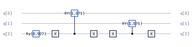
Piecewise-Linear Payoff Operator

PiecewiseLinearStateBlock is the piecewise-linear “payoff operator” of Woerner & Egger, npj Quantum Inf. 5, 15 (2019): from \(|0\rangle^{\otimes n}|0\rangle\) it puts the domain register in uniform superposition and rotates a flag qubit by an angle linear in \(x\) within each piece,

\[|0\ldots0\rangle \;\mapsto\; 2^{-n/2}\sum_{x=0}^{2^n-1} |x\rangle\bigl(\cos(\theta(x)/2)|0\rangle + \sin(\theta(x)/2)|1\rangle\bigr), \qquad \theta_i(x) = \text{slopes}_i\, x + \text{intercepts}_i \text{ for } x \text{ in piece } i.\]

The flag’s \(|1\rangle\) amplitude is what amplitude estimation reads out: with this block as the state-preparation operator, the estimated probability is \(2^{-n}\sum_x \sin^2(\theta(x)/2)\). The angle is linear in x, not the amplitude or the probability — callers wanting \(\sin^2(\theta/2) \approx f(x)\) choose slopes/intercepts under the small-angle convention of the amplitude-estimation literature themselves; the block is exact for whatever piecewise-linear \(\theta\) it is given.

The block is deterministic and control-safe: state_qubits are the domain qubits plus the flag, target_statevector() is the full column above on (domain..., flag) (LSB, index \(x + 2^n f\)), and the \(P - 1\) comparator ancillas that select the piece are uncomputed and return to \(|0\rangle\) with probability 1, so ancilla_postselection is None. It is therefore ready for AmplitudeEstimationBlock and safe under ControlledBlock. Whoever wants the postselected state \(\propto \sum_x \sin(\theta(x)/2)|x\rangle\) on the domain applies a PostSelection on the flag to a sampler result; the block itself never postselects.

Cost, measured as CNOTs on clifford_t_rz_gateset: 6 at \(n = 3, P = 1\); 100 at \(n = 3, P = 2\); 630 at \(n = 4, P = 3\); 5 970 at \(n = 6, P = 4\); 13 000–23 000 at \(n = 8, P = 4\) depending on the breakpoints’ bit patterns. Every rotation is controlled on all \(P - 1\) comparator bits plus a domain bit, and the prefix-match comparator is \(O(n^2)\) Toffolis per breakpoint. Woerner & Egger’s per-piece delta form (rotate by \(\text{slope}_i - \text{slope}_{i-1}\) controlled on comparator \(i\) alone, ≈ 700 CNOTs at \(n = 8, P = 4\)) and a ripple-carry comparator are declared follow-ups.

This block takes n_domain_qubits, breakpoints (the P - 1 interior breakpoints — integers, strictly ascending — splitting the domain into P pieces), and slopes/intercepts (length P each, radians).

from qarp import PostSelection
from qarp.blocks import PiecewiseLinearStateBlock

# Two pieces over an 8-value domain, split at x=3
state_block = PiecewiseLinearStateBlock(
    n_domain_qubits=3,
    breakpoints=[3],
    slopes=[0.1, 0.3],
    intercepts=[0.0, -0.2],
).build()

state_block.state_qubits              # the 3 domain qubits and the flag; the comparator is the ancilla
prepared, probability = state_block.prepared_statevector()
np.isclose(probability, 1.0)          # deterministic: nothing to postselect on

# The sin(theta/2)-weighted domain state is one postselection away
flag = state_block.state_qubits[-1]
payoff_branch = PostSelection({flag: 1})

A smaller instance, one breakpoint on a 2-qubit domain, keeps the comparator and controlled-rotation structure legible:

from qarp.blocks import PiecewiseLinearStateBlock

small_block = PiecewiseLinearStateBlock(
    n_domain_qubits=2,
    breakpoints=[1],
    slopes=[0.1, 0.3],
    intercepts=[0.0, -0.2],
).build()